
Featured Photo by Monstera on Pexels.
- In this post, we will put forward advanced integrated data visualization (AIDV) in the stock trading decisions and stock price prediction. The objective is to implement and visualize most popular stock technical indicators that are commonly used in technical analysis.
- From the point of view of algo trading, this study proves the credibility and advantages of AIDV in Python for the stock trading decisions and stock price prediction.
- Our final goal is to provide the trader with a dynamically changing and interactive UI using the technical analysis libraries available for Python and Plotly’s interactive AIDV tools.
In this project, we will implement the following Technical Indicators in Python:
- RSI, Volume (plain), Bollinger Bands, Aroon, Price Volume Trend, acceleration bands
- Stochastic, Chaikin Money Flow, Parabolic SAR, Rate of Change, Volume weighted average Price, momentum
- Commodity Channel Index, On Balance Volume, Keltner Channels, Triple Exponential Moving Average, Normalized Average True Range , directional movement indicators
- MACD, Money Flow index , Ichimoku, William %R, Volume MINMAX, adaptive moving average.
Conventionally, we will look at the following three main groups of technical indicators:
- Trend indicators — Simple Moving Average(SMA), Exponential Moving Average (EMA), Average Directional Movement Index (ADX), etc.
- Momentum indicators — Moving Average Convergence Divergence (MACD), Relative Strength Index (RSI), etc.
- Volatility indicators — e.g. Bollinger Bands.
Input Stock Data
Let’s set the working directory VIZ
import os
os.chdir(‘VIZ’)
os. getcwd()
and import the key libraries
import datetime as dt
import pandas as pd
import numpy as np
import matplotlib.pyplot as plt
import random
import copy
plt.style.use(‘fivethirtyeight’)
plt.rcParams[‘figure.figsize’] = (20,10)
Let’s download the stock data
def download_stock_data(ticker,timestamp_start,timestamp_end):
url=f”https://query1.finance.yahoo.com/v7/finance/download/{ticker}?period1={timestamp_start}&period2={timestamp_end}&interval\
=1d&events=history&includeAdjustedClose=true”
df = pd.read_csv(url)
return df
datetime_start=dt.datetime(2022, 1, 1, 7, 35, 51)
datetime_end=dt.datetime.today()
timestamp_start=int(datetime_start.timestamp())
timestamp_end=int(datetime_end.timestamp())
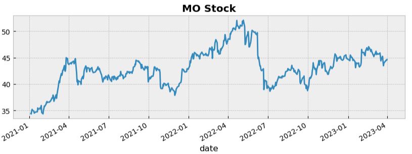
ticklist=[‘XOM’,’O’,’AZN’,’MO’,’COST’,’SBUX’,’AAPL’,’LMT’]
datac = []
for tick in ticklist:
df = download_stock_data(tick,timestamp_start,timestamp_end)
df = df.set_index(‘Date’)
df[‘Label’] = tick
datac.append(df)
print (datac)
[                  Open        High         Low       Close   Adj Close  \
Date
2022-01-03   61.240002   63.599998   61.209999   63.540001   60.648853
2022-01-04   64.129997   66.190002   64.099998   65.930000   62.930103
2022-01-05   66.500000   67.610001   66.480003   66.750000   63.712791
2022-01-06   68.000000   68.480003   67.070000   68.320000   65.211357
2022-01-07   68.519997   69.180000   67.980003   68.879997   65.745872
...                ...         ...         ...         ...         ...
2023-03-30  109.550003  109.570000  108.519997  109.489998  109.489998
2023-03-31  109.680000  110.169998  109.050003  109.660004  109.660004
2023-04-03  113.389999  116.849998  113.120003  116.129997  116.129997
2023-04-04  116.260002  116.699997  114.169998  115.019997  115.019997
2023-04-05  115.349998  117.000000  114.309998  116.989998  116.989998

              Volume Label
Date
2022-01-03  24282400   XOM
2022-01-04  38584000   XOM
2022-01-05  34033300   XOM
2022-01-06  30668500   XOM
2022-01-07  23985400   XOM
...              ...   ...
2023-03-30  11578200   XOM
2023-03-31  14416800   XOM
2023-04-03  28087700   XOM
2023-04-04  16365500   XOM
2023-04-05  16475200   XOM

[316 rows x 7 columns],                  Open       High        Low      Close  Adj Close   Volume  \
Date
2022-01-03  71.730003  71.809998  70.099998  71.199997  67.311935  3110500
2022-01-04  71.150002  72.480003  71.120003  72.250000  68.304596  3410700
2022-01-05  72.120003  72.480003  70.889999  71.080002  67.198494  3237600
2022-01-06  71.360001  71.870003  70.889999  71.410004  67.510460  2869800
2022-01-07  71.129997  71.540001  70.709999  71.410004  67.510460  3108900
...               ...        ...        ...        ...        ...      ...
2023-03-30  62.430000  62.860001  62.349998  62.610001  62.355000  3008000
2023-03-31  62.520000  63.360001  62.470001  63.320000  63.320000  4141500
2023-04-03  62.950001  63.400002  62.389999  62.869999  62.869999  5758400
2023-04-04  62.830002  62.990002  62.389999  62.840000  62.840000  2832400
2023-04-05  62.959999  63.110001  62.470001  62.709999  62.709999  4000600

           Label
Date
2022-01-03     O
2022-01-04     O
2022-01-05     O
2022-01-06     O
2022-01-07     O
...          ...
2023-03-30     O
2023-03-31     O
2023-04-03     O
2023-04-04     O
2023-04-05     O

[316 rows x 7 columns],                  Open       High        Low      Close  Adj Close   Volume  \
Date
2022-01-03  58.270000  58.369999  57.750000  58.310001  56.144096  3321000
2022-01-04  57.160000  57.700001  57.070000  57.270000  55.142727  4646600
2022-01-05  57.240002  57.730000  56.849998  56.880001  54.767216  4804400
2022-01-06  56.810001  57.040001  56.110001  56.669998  54.565006  6196400
2022-01-07  56.650002  57.549999  56.529999  57.480000  55.344921  4594800
...               ...        ...        ...        ...        ...      ...
2023-03-30  69.050003  69.220001  68.629997  69.199997  69.199997  4648100
2023-03-31  69.879997  69.930000  69.239998  69.410004  69.410004  3500300
2023-04-03  69.529999  69.949997  69.360001  69.910004  69.910004  4749200
2023-04-04  69.980003  70.570000  69.809998  70.250000  70.250000  4383400
2023-04-05  72.000000  72.480003  71.800003  72.050003  72.050003  5873200

           Label
Date
2022-01-03   AZN
2022-01-04   AZN
2022-01-05   AZN
2022-01-06   AZN
2022-01-07   AZN
...          ...
2023-03-30   AZN
2023-03-31   AZN
2023-04-03   AZN
2023-04-04   AZN
2023-04-05   AZN

[316 rows x 7 columns],                  Open       High        Low      Close  Adj Close    Volume  \
Date
2022-01-03  47.369999  48.000000  47.180000  47.970001  43.408066  10308100
2022-01-04  48.000000  49.340000  47.980000  49.029999  44.367256  11647900
2022-01-05  48.549999  49.270000  48.330002  48.639999  44.014351  11506500
2022-01-06  49.180000  49.720001  48.869999  49.209999  44.530140  10134100
2022-01-07  49.200001  50.000000  49.099998  49.770000  45.036888   8098600
...               ...        ...        ...        ...        ...       ...
2023-03-30  44.639999  44.830002  44.349998  44.500000  44.500000   6862400
2023-03-31  44.630001  44.720001  44.430000  44.619999  44.619999   7710000
2023-04-03  44.720001  45.330002  44.599998  44.980000  44.980000   8385800
2023-04-04  44.880001  44.910000  44.240002  44.450001  44.450001   7379600
2023-04-05  44.459999  44.700001  44.189999  44.430000  44.430000   7865000

           Label
Date
2022-01-03    MO
2022-01-04    MO
2022-01-05    MO
2022-01-06    MO
2022-01-07    MO
...          ...
2023-03-30    MO
2023-03-31    MO
2023-04-03    MO
2023-04-04    MO
2023-04-05    MO

[316 rows x 7 columns],                   Open        High         Low       Close   Adj Close  \
Date
2022-01-03  565.030029  567.469971  555.510010  566.710022  561.965271
2022-01-04  564.229980  568.719971  561.789978  564.229980  559.506042
2022-01-05  563.690002  565.049988  549.770020  549.919983  545.315857
2022-01-06  546.200012  553.520020  543.549988  549.799988  545.196899
2022-01-07  547.549988  548.369995  534.239990  536.179993  531.690857
...                ...         ...         ...         ...         ...
2023-03-30  493.000000  495.739990  491.000000  491.480011  491.480011
2023-03-31  495.000000  498.359985  493.940002  496.869995  496.869995
2023-04-03  496.500000  499.200012  495.000000  497.029999  497.029999
2023-04-04  496.500000  502.579987  495.500000  497.730011  497.730011
2023-04-05  499.000000  504.130005  495.160004  497.130005  497.130005

             Volume Label
Date
2022-01-03  2714100  COST
2022-01-04  2097500  COST
2022-01-05  2887500  COST
2022-01-06  2503100  COST
2022-01-07  2323900  COST
...             ...   ...
2023-03-30  1545500  COST
2023-03-31  2081300  COST
2023-04-03  1804700  COST
2023-04-04  1913300  COST
2023-04-05  1930600  COST

[316 rows x 7 columns],                   Open        High         Low       Close   Adj Close  \
Date
2022-01-03  116.470001  117.800003  114.779999  116.680000  113.403084
2022-01-04  116.900002  117.050003  114.169998  114.239998  111.031593
2022-01-05  114.400002  114.959999  110.400002  110.440002  107.338318
2022-01-06  110.000000  111.879997  109.989998  111.139999  108.018661
2022-01-07  108.220001  109.709999  107.480003  107.570000  104.548920
...                ...         ...         ...         ...         ...
2023-03-30  101.440002  101.699997  100.650002  101.320000  101.320000
2023-03-31  101.839996  104.279999  101.839996  104.129997  104.129997
2023-04-03  104.059998  104.940002  103.669998  104.849998  104.849998
2023-04-04  104.849998  105.010002  103.349998  104.000000  104.000000
2023-04-05  103.980003  105.699997  103.930000  104.900002  104.900002

              Volume Label
Date
2022-01-03   5475700  SBUX
2022-01-04   8367600  SBUX
2022-01-05   8662300  SBUX
2022-01-06   6099900  SBUX
2022-01-07  11266400  SBUX
...              ...   ...
2023-03-30   4082600  SBUX
2023-03-31   6899300  SBUX
2023-04-03   3855400  SBUX
2023-04-04   3854400  SBUX
2023-04-05   5169900  SBUX

[316 rows x 7 columns],                   Open        High         Low       Close   Adj Close  \
Date
2022-01-03  177.830002  182.880005  177.710007  182.009995  180.683868
2022-01-04  182.630005  182.940002  179.119995  179.699997  178.390701
2022-01-05  179.610001  180.169998  174.639999  174.919998  173.645538
2022-01-06  172.699997  175.300003  171.639999  172.000000  170.746826
2022-01-07  172.889999  174.139999  171.029999  172.169998  170.915588
...                ...         ...         ...         ...         ...
2023-03-30  161.529999  162.470001  161.270004  162.360001  162.360001
2023-03-31  162.440002  165.000000  161.910004  164.899994  164.899994
2023-04-03  164.270004  166.289993  164.220001  166.169998  166.169998
2023-04-04  166.600006  166.839996  165.110001  165.630005  165.630005
2023-04-05  164.740005  165.050003  161.800003  163.759995  163.759995

               Volume Label
Date
2022-01-03  104487900  AAPL
2022-01-04   99310400  AAPL
2022-01-05   94537600  AAPL
2022-01-06   96904000  AAPL
2022-01-07   86709100  AAPL
...               ...   ...
2023-03-30   49501700  AAPL
2023-03-31   68694700  AAPL
2023-04-03   56976200  AAPL
2023-04-04   46278300  AAPL
2023-04-05   51457200  AAPL

[316 rows x 7 columns],                   Open        High         Low       Close   Adj Close  \
Date
2022-01-03  354.679993  356.589996  353.029999  354.359985  343.132660
2022-01-04  355.529999  363.540009  355.209991  361.989990  350.520935
2022-01-05  363.000000  364.000000  357.869995  358.140015  346.792938
2022-01-06  360.000000  361.239990  357.549988  358.000000  346.657349
2022-01-07  359.079987  362.989990  358.149994  360.140015  348.729553
...                ...         ...         ...         ...         ...
2023-03-30  474.540009  475.799988  471.730011  473.179993  473.179993
2023-03-31  474.190002  475.350006  471.029999  472.730011  472.730011
2023-04-03  473.000000  487.899994  472.750000  486.619995  486.619995
2023-04-04  485.589996  490.630005  484.750000  488.540009  488.540009
2023-04-05  488.000000  493.829987  487.029999  489.989990  489.989990

             Volume Label
Date
2022-01-03  1205700   LMT
2022-01-04  1361100   LMT
2022-01-05  1682200   LMT
2022-01-06  1368800   LMT
2022-01-07  1634600   LMT
...             ...   ...
2023-03-30   950300   LMT
2023-03-31  1409600   LMT
2023-04-03  1656700   LMT
2023-04-04  1081100   LMT
2023-04-05  1305500   LMT

[316 rows x 7 columns]]
TechIndicator = copy.deepcopy(data)
Relative Strength Index (RSI)
- The relative strength index (RSI) is a momentum indicator used in technical analysis. RSI measures the speed and magnitude of a security’s recent price changes to evaluate overvalued or undervalued conditions in the price of that security.
- The RSI is displayed as an oscillator (a line graph) on a scale of zero to 100.
- An asset is usually considered overbought when the RSI is above 70 and oversold when it is below 30.
def rsi(values):
up = values[values>0].mean()
down = -1*values[values<0].mean()
return 100 * up / (up + down)
for stock in range(len(TechIndicator)):
TechIndicator[stock][‘Momentum_1D’] = (TechIndicator[stock][‘Close’]-TechIndicator[stock][‘Close’].shift(1)).fillna(0)
TechIndicator[stock][‘RSI_14D’] = TechIndicator[stock][‘Momentum_1D’].rolling(center=False, window=14).apply(rsi).fillna(0)
TechIndicator[0].tail(5)
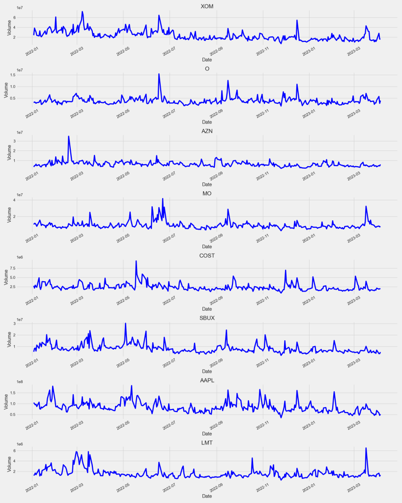
Volume
- Trading volume is a measure of how much a given financial asset has traded in a period of time. For stocks, volume is measured in the number of shares traded. For futures and options, volume is based on how many contracts have changed hands. Traders look to volume to determine liquidity and combine changes in volume with technical indicators to make trading decisions.
- Volume measures the number of shares traded in a stock or contracts traded in futures or options.
- Volume can indicate market strength, as rising markets on increasing volume are typically viewed as strong and healthy.
- When prices fall on increasing volume, the trend is gathering strength to the downside.
- When prices reach new highs (or no lows) on decreasing volume, watch out—a reversal might be taking shape.
- On-balance volume (OBV) and the Klinger oscillator are examples of charting tools that are based on volume.
for stock in range(len(TechIndicator)):
TechIndicator[stock][‘Volume_plain’] = TechIndicator[stock][‘Volume’].fillna(0)
TechIndicator[0].tail()
Bollinger Bands (BB)
- Bollinger Bands® is a technical analysis tool to generate oversold or overbought signals and was developed by John Bollinger.
- Three lines compose Bollinger Bands: A simple moving average, or the middle band, and an upper and lower band.
- The upper and lower bands are typically 2 standard deviations +/- from a 20-day simple moving average and can be modified.
- When the price continually touches the upper Bollinger Band, it can indicate an overbought signal.
- If the price continually touches the lower band it can indicate an oversold signal.
def bbands(price, length=30, numsd=2):
“”” returns average, upper band, and lower band”””
#ave = pd.stats.moments.rolling_mean(price,length)
ave = price.rolling(window = length, center = False).mean()
#sd = pd.stats.moments.rolling_std(price,length)
sd = price.rolling(window = length, center = False).std()
upband = ave + (sdnumsd) dnband = ave – (sdnumsd)
return np.round(ave,3), np.round(upband,3), np.round(dnband,3)
for stock in range(len(TechIndicator)):
TechIndicator[stock][‘BB_Middle_Band’], TechIndicator[stock][‘BB_Upper_Band’], TechIndicator[stock][‘BB_Lower_Band’] = bbands(TechIndicator[stock][‘Close’], length=20, numsd=1)
TechIndicator[stock][‘BB_Middle_Band’] = TechIndicator[stock][‘BB_Middle_Band’].fillna(0)
TechIndicator[stock][‘BB_Upper_Band’] = TechIndicator[stock][‘BB_Upper_Band’].fillna(0)
TechIndicator[stock][‘BB_Lower_Band’] = TechIndicator[stock][‘BB_Lower_Band’].fillna(0)
TechIndicator[0].tail()
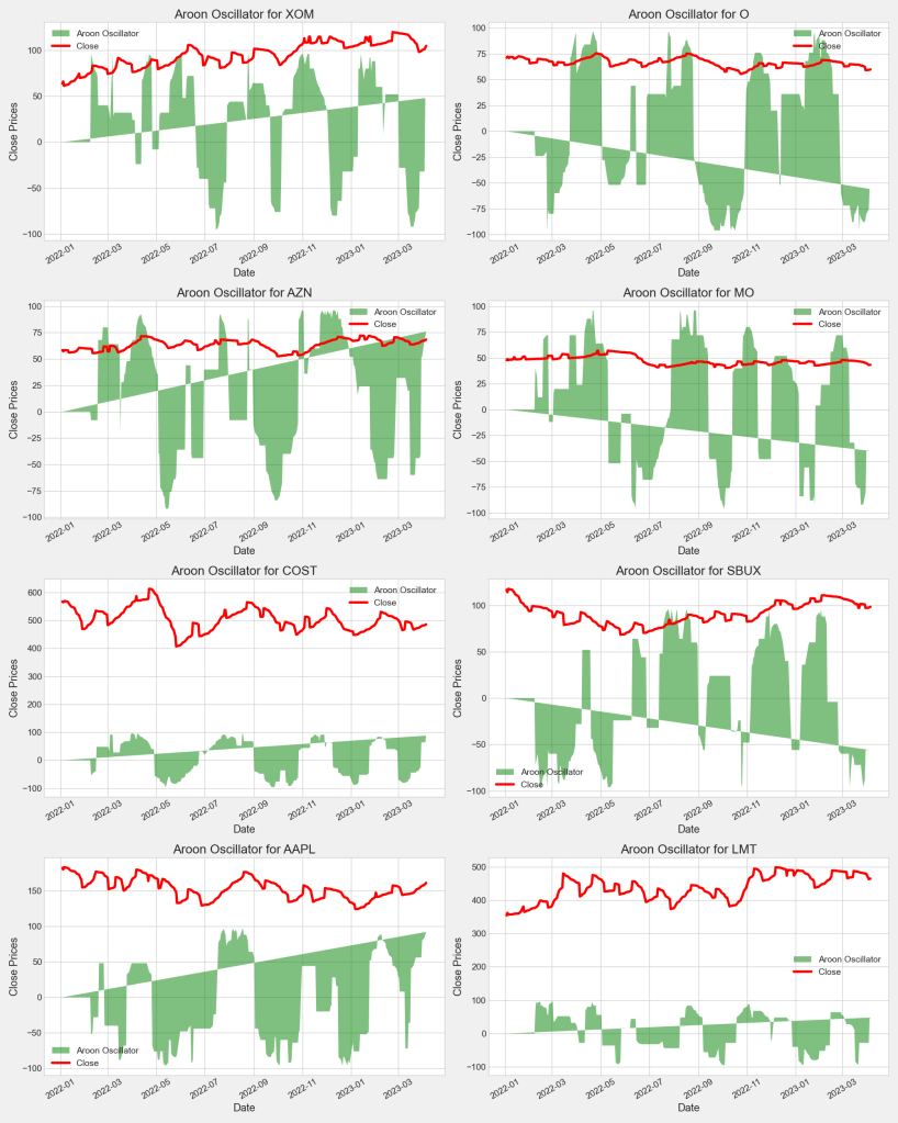
Aroon Oscillator (AO)
The Aroon indicator is a technical indicator that is used to identify trend changes in the price of an asset, as well as the strength of that trend.
- The Aroon indicator is composed of two lines. An up line which measures the number of periods since a High, and a down line which measures the number of periods since a Low.
- The indicator is typically applied to 25 periods of data, so the indicator is showing how many periods it has been since a 25-period high or low.
- When the Aroon Up is above the Aroon Down, it indicates bullish price behavior.
- When the Aroon Down is above the Aroon Up, it signals bearish price behavior.
- Crossovers of the two lines can signal trend changes. For example, when Aroon Up crosses above Aroon Down it may mean a new uptrend is starting.
- The indicator moves between zero and 100.
def aroon(df, tf=25):
aroonup = []
aroondown = []
x = tf
while x< len(df.index):
aroon_up = ((df[‘High’][x-tf:x].tolist().index(max(df[‘High’][x-tf:x])))/float(tf))100 aroon_down = ((df[‘Low’][x-tf:x].tolist().index(min(df[‘Low’][x-tf:x])))/float(tf))100
aroonup.append(aroon_up)
aroondown.append(aroon_down)
x+=1
return aroonup, aroondown
for stock in range(len(TechIndicator)):
listofzeros = [0] * 25
up, down = aroon(TechIndicator[stock])
aroon_list = [x – y for x, y in zip(up,down)]
if len(aroon_list)==0:
aroon_list = [0] * TechIndicator[stock].shape[0]
TechIndicator[stock][‘Aroon_Oscillator’] = aroon_list
else:
TechIndicator[stock][‘Aroon_Oscillator’] = listofzeros+aroon_list
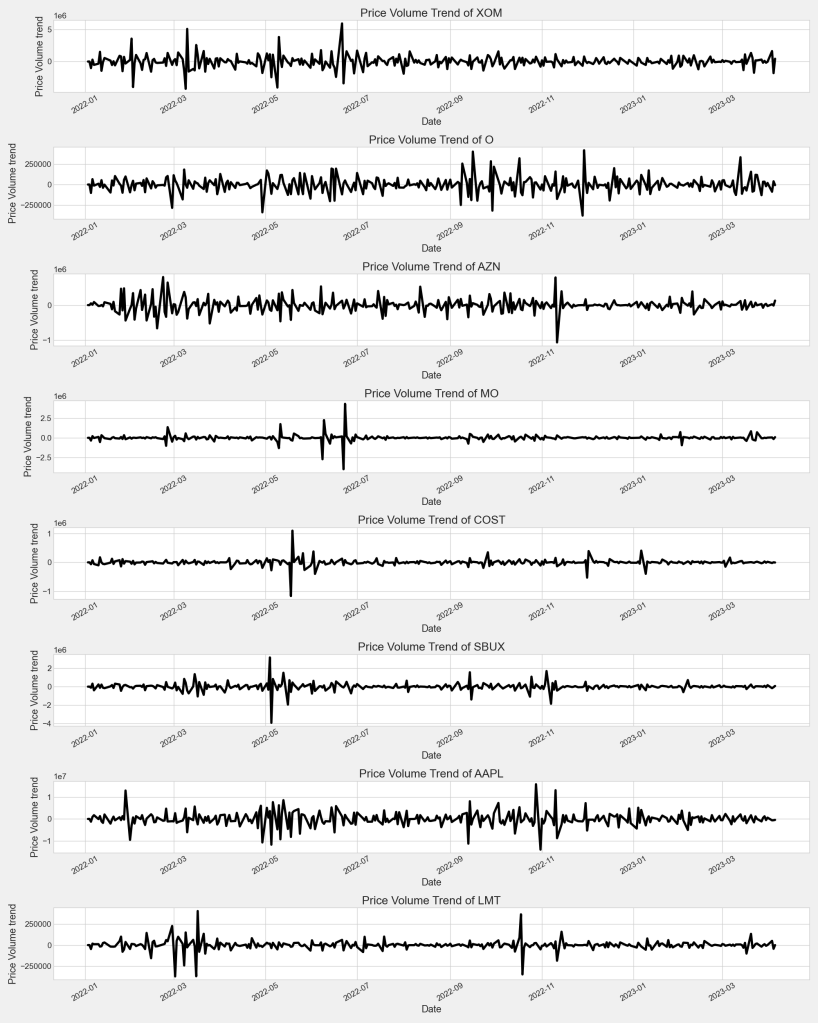
Price Volume Trend (PVT)
The PVT indicator helps determine a security’s price direction and strength of price change. The indicator consists of a cumulative volume line that adds or subtracts a multiple of the percentage change in a share prices’ trend and current volume, depending upon the security’s upward or downward movements.
for stock in range(len(TechIndicator)):
TechIndicator[stock][“PVT”] = (TechIndicator[stock][‘Momentum_1D’]/ TechIndicator[stock][‘Close’].shift(1))*TechIndicator[stock][‘Volume’]
TechIndicator[stock][“PVT”] = TechIndicator[stock][“PVT”]-TechIndicator[stock][“PVT”].shift(1)
TechIndicator[stock][“PVT”] = TechIndicator[stock][“PVT”].fillna(0)
TechIndicator[0].tail()
Acceleration Bands (AB)
The Acceleration Bands measure volatility over a user-defined number of bars (default is often the past 20 bars). They are plotted using a simple moving average as the midpoint, with the upper and lower bands being of equal distance from the midpoint, similar to Bollinger Bands.
def abands(df):
#df[‘AB_Middle_Band’] = pd.rolling_mean(df[‘Close’], 20)
df[‘AB_Middle_Band’] = df[‘Close’].rolling(window = 20, center=False).mean()
# High * ( 1 + 4 * (High – Low) / (High + Low))
df[‘aupband’] = df[‘High’] * (1 + 4 * (df[‘High’]-df[‘Low’])/(df[‘High’]+df[‘Low’]))
df[‘AB_Upper_Band’] = df[‘aupband’].rolling(window=20, center=False).mean()
# Low *(1 – 4 * (High – Low)/ (High + Low))
df[‘adownband’] = df[‘Low’] * (1 – 4 * (df[‘High’]-df[‘Low’])/(df[‘High’]+df[‘Low’]))
df[‘AB_Lower_Band’] = df[‘adownband’].rolling(window=20, center=False).mean()
for stock in range(len(TechIndicator)):
abands(TechIndicator[stock])
TechIndicator[stock] = TechIndicator[stock].fillna(0)
TechIndicator[0].tail()
columns2Drop = [‘Momentum_1D’, ‘aupband’, ‘adownband’]
for stock in range(len(TechIndicator)):
TechIndicator[stock] = TechIndicator[stock].drop(labels = columns2Drop, axis=1)
TechIndicator[0].head()
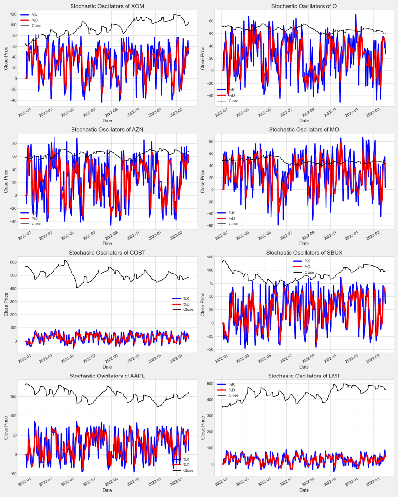
Stochastic Oscillator (%K and %D)
A stochastic oscillator is a momentum indicator comparing a particular closing price of a security to a range of its prices over a certain period of time. The sensitivity of the oscillator to market movements is reducible by adjusting that time period or by taking a moving average of the result. It is used to generate overbought and oversold trading signals, utilizing a 0–100 bounded range of values.
- Stochastics are a favored technical indicator because they are easy to understand and have a relatively high degree of accuracy.
- It falls into the class of technical indicators known as oscillators.
- The indicator provides buy and sell signals for traders to enter or exit positions based on momentum.
- Stochastics are used to show when a stock has moved into an overbought or oversold position.
- it is beneficial to use stochastics in conjunction with other tools like the relative strength index (RSI) to confirm a signal.
def STOK(df, n):
df[‘STOK’] = ((df[‘Close’] – df[‘Low’].rolling(window=n, center=False).mean()) / (df[‘High’].rolling(window=n, center=False).max() – df[‘Low’].rolling(window=n, center=False).min())) * 100
df[‘STOD’] = df[‘STOK’].rolling(window = 3, center=False).mean()
for stock in range(len(TechIndicator)):
STOK(TechIndicator[stock], 4)
TechIndicator[stock] = TechIndicator[stock].fillna(0)
TechIndicator[0].tail()
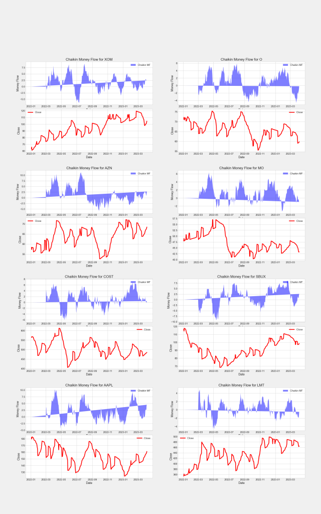
Chaikin Money Flow (CMFlow)
- The Chaikin Indicator applies MACD to the accumulation-distribution line rather than to the closing price.
- It is an oscillator technical indicator for spotting trends and reversals.
- A cross above the accumulation-distribution line indicates that market players are accumulating shares, securities, or contracts, which is typically bullish.
To calculate the Chaikin oscillator, subtract a 10-day exponential moving average (EMA) of the accumulation-distribution line from a 3-day EMA of the accumulation-distribution line. This measures momentum predicted by oscillations around the accumulation-distribution line.
def CMFlow(df, tf):
CHMF = []
MFMs = []
MFVs = []
x = tf
while x < len(df.index):
    PeriodVolume = 0
    volRange = df['Volume'][x-tf:x]
    for eachVol in volRange:
        PeriodVolume += eachVol

    MFM = ((df['Close'][x] - df['Low'][x]) - (df['High'][x] - df['Close'][x])) / (df['High'][x] - df['Low'][x])
    MFV = MFM*PeriodVolume

    MFMs.append(MFM)
    MFVs.append(MFV)
    x+=1

y = tf
while y < len(MFVs):
    PeriodVolume = 0
    volRange = df['Volume'][x-tf:x]
    for eachVol in volRange:
        PeriodVolume += eachVol
    consider = MFVs[y-tf:y]
    tfsMFV = 0

    for eachMFV in consider:
        tfsMFV += eachMFV

    tfsCMF = tfsMFV/PeriodVolume
    CHMF.append(tfsCMF)
    y+=1
return CHMF
for stock in range(len(TechIndicator)):
listofzeros = [0] * 40
CHMF = CMFlow(TechIndicator[stock], 20)
if len(CHMF)==0:
CHMF = [0] * TechIndicator[stock].shape[0]
TechIndicator[stock][‘Chaikin_MF’] = CHMF
else:
TechIndicator[stock][‘Chaikin_MF’] = listofzeros+CHMF
TechIndicator[0].tail()
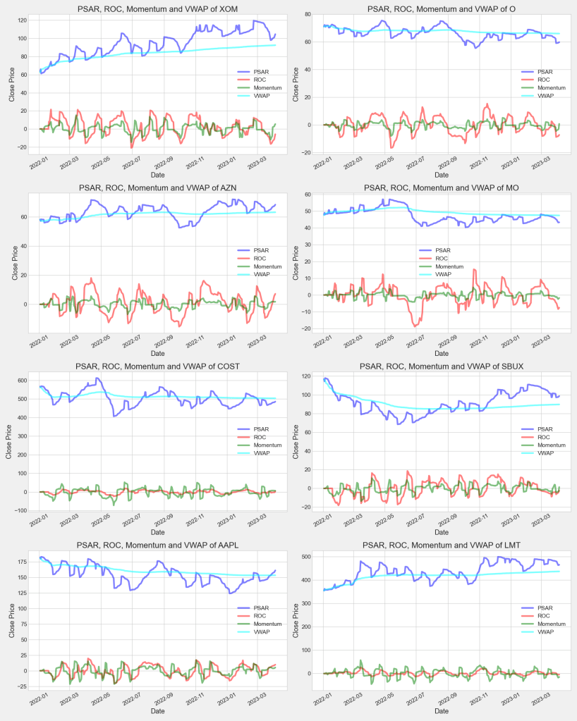
Parabolic SAR (PSAR)
- The parabolic SAR indicator appears on a chart as a series of dots, either above or below an asset’s price, depending on the direction the price is moving. A dot is placed below the price when it is trending upward, and above the price when it is trending downward.
- A reversal occurs when these dots flip, but a reversal signal in the SAR does not necessarily mean a reversal in the price. A PSAR reversal only means that the price and indicator have crossed.
def psar(df, iaf = 0.02, maxaf = 0.2):
length = len(df)
dates = (df.index)
high = (df[‘High’])
low = (df[‘Low’])
close = (df[‘Close’])
psar = df[‘Close’][0:len(df[‘Close’])]
psarbull = [None] * length
psarbear = [None] * length
bull = True
af = iaf
ep = df[‘Low’][0]
hp = df[‘High’][0]
lp = df[‘Low’][0]
for i in range(2,length):
if bull:
psar[i] = psar[i – 1] + af * (hp – psar[i – 1])
else:
psar[i] = psar[i – 1] + af * (lp – psar[i – 1])
reverse = False
if bull:
if df[‘Low’][i] < psar[i]: bull = False reverse = True psar[i] = hp lp = df[‘Low’][i] af = iaf else: if df[‘High’][i] > psar[i]:
bull = True
reverse = True
psar[i] = lp
hp = df[‘High’][i]
af = iaf
if not reverse:
if bull:
if df[‘High’][i] > hp:
hp = df[‘High’][i]
af = min(af + iaf, maxaf)
if df[‘Low’][i – 1] < psar[i]: psar[i] = df[‘Low’][i – 1] if df[‘Low’][i – 2] < psar[i]: psar[i] = df[‘Low’][i – 2] else: if df[‘Low’][i] < lp: lp = df[‘Low’][i] af = min(af + iaf, maxaf) if df[‘High’][i – 1] > psar[i]:
psar[i] = df[‘High’][i – 1]
if df[‘High’][i – 2] > psar[i]:
psar[i] = df[‘High’][i – 2]
if bull:
psarbull[i] = psar[i]
else:
psarbear[i] = psar[i]
df[‘psar’] = psar
for stock in range(len(TechIndicator)):
psar(TechIndicator[stock])
TechIndicator[0].tail()
Price Rate of Change (ROC)
The Price Rate of Change (ROC) is a momentum-based technical indicator that measures the percentage change in price between the current price and the price a certain number of periods ago. The ROC indicator is plotted against zero, with the indicator moving upwards into positive territory if price changes are to the upside, and moving into negative territory if price changes are to the downside.
- The Price Rate of Change (ROC) oscillator is an unbounded momentum indicator used in technical analysis set against a zero-level midpoint.
- A rising ROC above zero typically confirms an uptrend while a falling ROC below zero indicates a downtrend.
- When the price is consolidating, the ROC will hover near zero. In this case, it is important traders watch the overall price trend since the ROC will provide little insight except for confirming the consolidation.
# ROC = [(Close – Close n periods ago) / (Close n periods ago)] * 100
for stock in range(len(TechIndicator)):
TechIndicator[stock][‘ROC’] = ((TechIndicator[stock][‘Close’] – TechIndicator[stock][‘Close’].shift(12))/(TechIndicator[stock][‘Close’].shift(12)))*100
TechIndicator[stock] = TechIndicator[stock].fillna(0)
TechIndicator[0].tail()
Volume Weighted Average Price (VWAP)
- The VWAP is a technical analysis indicator used on intraday charts that resets at the start of every new trading session.
- It’s a trading benchmark that represents the average price a security has traded at throughout the day, based on both volume and price.
- VWAP appears as a single line on intraday charts.
- It looks similar to a moving average line, but smoother.
- VWAP represents a view of price action throughout a single day’s trading session.
- Retail and professional traders may use VWAP to help them determine intraday price trends.
- VWAP typically is most useful to short-term traders.
for stock in range(len(TechIndicator)):
TechIndicator[stock][‘VWAP’] = np.cumsum(TechIndicator[stock][‘Volume’] * (TechIndicator[stock][‘High’] + TechIndicator[stock][‘Low’])/2) / np.cumsum(TechIndicator[stock][‘Volume’])
TechIndicator[stock] = TechIndicator[stock].fillna(0)
TechIndicator[0].tail()
Momentum
Momentum measures the rate of the rise or fall in stock prices. For trending analysis, momentum is a useful indicator of strength or weakness in the issue’s price. History has shown that momentum is far more useful during rising markets than falling markets because markets rise more often than they fall.
for stock in range(len(TechIndicator)):
TechIndicator[stock][‘Momentum’] = TechIndicator[stock][‘Close’] – TechIndicator[stock][‘Close’].shift(4)
TechIndicator[stock] = TechIndicator[stock].fillna(0)
TechIndicator[0].tail()
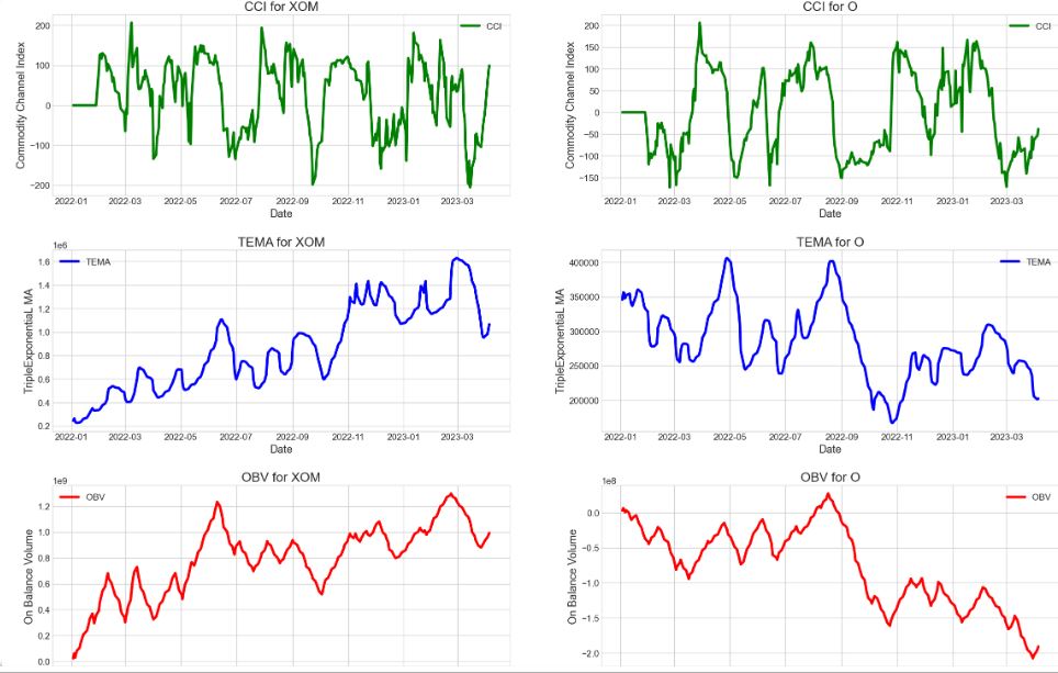
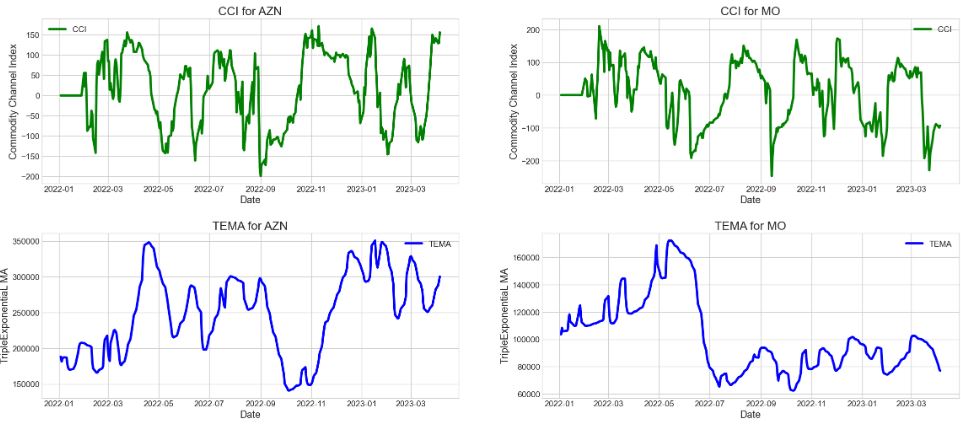
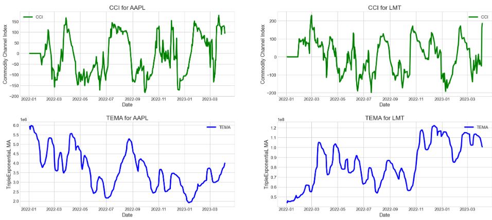
Commodity Channel Index (CCI)
- The Commodity Channel Index (CCI) is a technical indicator that measures the difference between the current price and the historical average price.
- When the CCI is above zero, it indicates the price is above the historic average. Conversely, when the CCI is below zero, the price is below the historic average.
- The CCI is an unbounded oscillator, meaning it can go higher or lower indefinitely. For this reason, overbought and oversold levels are typically determined for each individual asset by looking at historical extreme CCI levels where the price reversed from.
def CCI(df, n, constant):
TP = (df[‘High’] + df[‘Low’] + df[‘Close’]) / 3
CCI = pd.Series((TP – TP.rolling(window=n, center=False).mean()) / (constant * TP.rolling(window=n, center=False).std())) #, name = ‘CCI_’ + str(n))
return CCI
for stock in range(len(TechIndicator)):
TechIndicator[stock][‘CCI’] = CCI(TechIndicator[stock], 20, 0.015)
TechIndicator[stock] = TechIndicator[stock].fillna(0)
TechIndicator[0].tail()
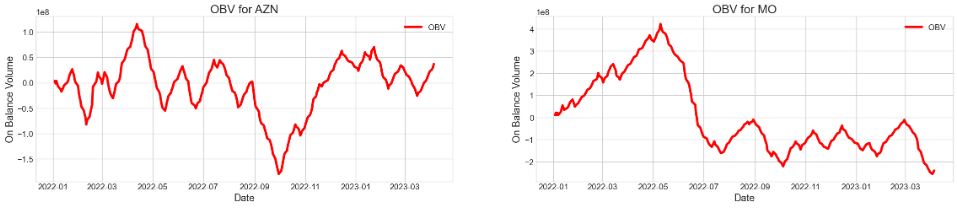
On Balance Volume (OBV)
On-balance volume (OBV) is a technical trading momentum indicator that uses volume flow to predict changes in stock price.
- OBV shows crowd sentiment that can predict a bullish or bearish outcome.
- Comparing relative action between price bars and OBV generates more actionable signals than the green or red volume histograms commonly found at the bottom of price charts.
for stock in range(len(TechIndicator)):
new = (TechIndicator[stock][‘Volume’] * (~TechIndicator[stock][‘Close’].diff().le(0) * 2 -1)).cumsum()
TechIndicator[stock][‘OBV’] = new
TechIndicator[5].tail()
Keltner Channels (KCH)
- Keltner Channels are volatility-based bands that are placed on either side of an asset’s price and can aid in determining the direction of a trend.
- The exponential moving average (EMA) of a Keltner Channel is typically 20 periods, although this can be adjusted if desired.
- The upper and lower bands are typically set two times the average true range (ATR) above and below the EMA, although the multiplier can also be adjusted based on personal preference.
- Price reaching the upper Keltner Channel band is bullish, while reaching the lower band is bearish.
- The angle of the Keltner Channel also aids in identifying the trend direction. The price may also oscillate between the upper and lower Keltner Channel bands, which can be interpreted as resistance and support levels.
def KELCH(df, n):
KelChM = pd.Series(((df[‘High’] + df[‘Low’] + df[‘Close’]) / 3).rolling(window =n, center=False).mean(), name = ‘KelChM_’ + str(n))
KelChU = pd.Series(((4 * df[‘High’] – 2 * df[‘Low’] + df[‘Close’]) / 3).rolling(window =n, center=False).mean(), name = ‘KelChU_’ + str(n))
KelChD = pd.Series(((-2 * df[‘High’] + 4 * df[‘Low’] + df[‘Close’]) / 3).rolling(window =n, center=False).mean(), name = ‘KelChD_’ + str(n))
return KelChM, KelChD, KelChU
for stock in range(len(TechIndicator)):
KelchM, KelchD, KelchU = KELCH(TechIndicator[stock], 14)
TechIndicator[stock][‘Kelch_Upper’] = KelchU
TechIndicator[stock][‘Kelch_Middle’] = KelchM
TechIndicator[stock][‘Kelch_Down’] = KelchD
TechIndicator[stock] = TechIndicator[stock].fillna(0)
TechIndicator[5].tail()
Triple Exponential Moving Average (TEMA)
- The triple exponential moving average (TEMA) uses multiple EMA calculations and subtracts out the lag to create a trend following indicator that reacts quickly to price changes.
- The TEMA indicator can help identify trend direction, signal potential short-term trend changes or pullbacks, and provide support or resistance.
- When the price is above the TEMA it helps confirm an uptrend; when the price is below the TEMA it helps confirm a downtrend.
for stock in range(len(TechIndicator)):
TechIndicator[stock][‘EMA’] = TechIndicator[stock][‘Close’].ewm(span=3,min_periods=0,adjust=True,ignore_na=False).mean()
TechIndicator[stock] = TechIndicator[stock].fillna(0)
for stock in range(len(TechIndicator)):
TechIndicator[stock][‘TEMA’] = (3 * TechIndicator[stock][‘EMA’] – 3 * TechIndicator[stock][‘EMA’] * TechIndicator[stock][‘EMA’]) + (TechIndicator[stock][‘EMA’]TechIndicator[stock][‘EMA’]TechIndicator[stock][‘EMA’])
TechIndicator[5].tail()
Normalized Average True Range (NATR)
- The average true range (ATR) is a market volatility indicator used in technical analysis.
- It is typically derived from the 14-day simple moving average of a series of true range indicators.
- The ATR was initially developed for use in commodities markets but has since been applied to all types of securities.
- ATR shows investors the average range prices swing for an investment over a specified period.
- True Range = Highest of (HIgh – low, abs(High – previous close), abs(low – previous close))
- Average True Range = 14 day MA of True Range
- Normalized Average True Range = ATR / Close * 100
for stock in range(len(TechIndicator)):
TechIndicator[stock][‘HL’] = TechIndicator[stock][‘High’] – TechIndicator[stock][‘Low’]
TechIndicator[stock][‘absHC’] = abs(TechIndicator[stock][‘High’] – TechIndicator[stock][‘Close’].shift(1))
TechIndicator[stock][‘absLC’] = abs(TechIndicator[stock][‘Low’] – TechIndicator[stock][‘Close’].shift(1))
TechIndicator[stock][‘TR’] = TechIndicator[stock][[‘HL’,’absHC’,’absLC’]].max(axis=1)
TechIndicator[stock][‘ATR’] = TechIndicator[stock][‘TR’].rolling(window=14).mean()
TechIndicator[stock][‘NATR’] = (TechIndicator[stock][‘ATR’] / TechIndicator[stock][‘Close’]) *100
TechIndicator[stock] = TechIndicator[stock].fillna(0)
TechIndicator[5].tail()
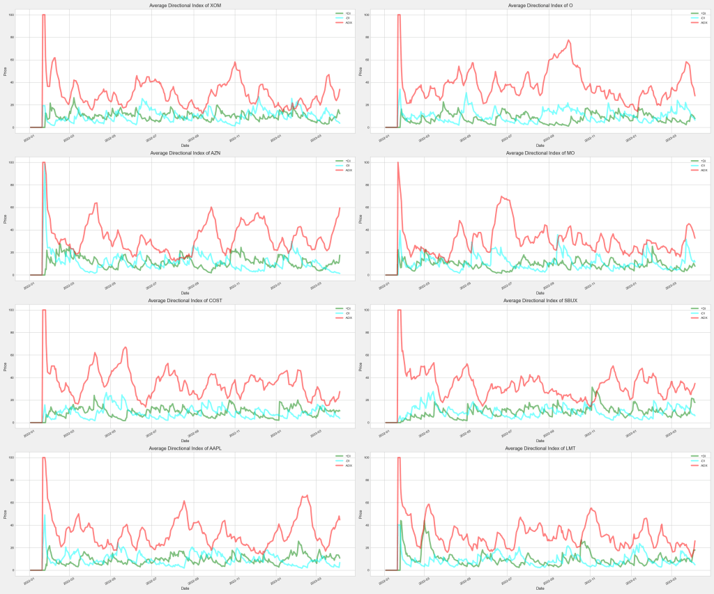
Average Directional Movement Index (ADX)
The average directional index (ADX) helps traders see the trend direction as well as the strength of that trend. The Positive Directional Indicator (+DI) is one of the lines in the Average Directional Index (ADX) indicator and is used to measure the presence of an uptrend.
- The ADX is now used in several markets by technical traders to judge the strength of a trend.
- The ADX makes use of a positive (+DI) and negative (-DI) directional indicator in addition to the trendline.
- The trend has strength when ADX is above 25; the trend is weak or the price is trendless when ADX is below 20, according to Wilder.
- Non-trending doesn’t mean the price isn’t moving. It may not be, but the price could also be making a trend change or is too volatile for a clear direction to be present.
def DMI(df, period):
df[‘UpMove’] = df[‘High’] – df[‘High’].shift(1)
df[‘DownMove’] = df[‘Low’].shift(1) – df[‘Low’]
df[‘Zero’] = 0
df['PlusDM'] = np.where((df['UpMove'] > df['DownMove']) & (df['UpMove'] > df['Zero']), df['UpMove'], 0)
df['MinusDM'] = np.where((df['UpMove'] < df['DownMove']) & (df['DownMove'] > df['Zero']), df['DownMove'], 0)

df['plusDI'] = 100 * (df['PlusDM']/df['ATR']).ewm(span=period,min_periods=0,adjust=True,ignore_na=False).mean()
df['minusDI'] = 100 * (df['MinusDM']/df['ATR']).ewm(span=period,min_periods=0,adjust=True,ignore_na=False).mean()

df['ADX'] = 100 * (abs((df['plusDI'] - df['minusDI'])/(df['plusDI'] + df['minusDI']))).ewm(span=period,min_periods=0,adjust=True,ignore_na=False).mean()
for stock in range(len(TechIndicator)):
DMI(TechIndicator[stock], 14)
TechIndicator[stock] = TechIndicator[stock].fillna(0)
TechIndicator[5].tail()
columns2Drop = [‘UpMove’, ‘DownMove’, ‘ATR’, ‘PlusDM’, ‘MinusDM’, ‘Zero’, ‘EMA’, ‘HL’, ‘absHC’, ‘absLC’, ‘TR’]
for stock in range(len(TechIndicator)):
TechIndicator[stock] = TechIndicator[stock].drop(labels = columns2Drop, axis=1)
TechIndicator[2].head()
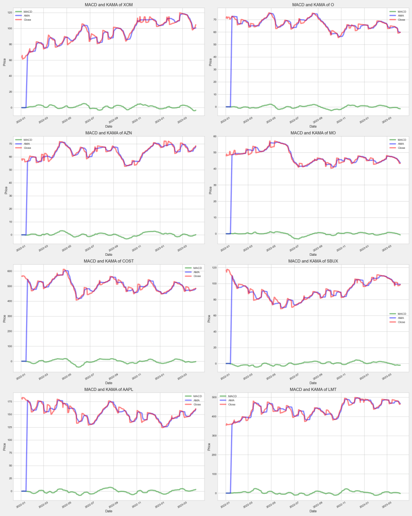
MACD
- Moving average convergence/divergence (MACD, or MAC-D) is a trend-following momentum indicator that shows the relationship between two exponential moving averages (EMAs) of a security’s price. The MACD line is calculated by subtracting the 26-period EMA from the 12-period EMA.
- The result of that calculation is the MACD line. A nine-day EMA of the MACD line is called the signal line, which is then plotted on top of the MACD line, which can function as a trigger for buy or sell signals.
- Traders may buy the security when the MACD line crosses above the signal line and sell—or short—the security when the MACD line crosses below the signal line. MACD indicators can be interpreted in several ways, but the more common methods are crossovers, divergences, and rapid rises/falls.
- MACD is best used with daily periods, where the traditional settings of 26/12/9 days is the norm.
- MACD triggers technical signals when the MACD line crosses above the signal line (to buy) or falls below it (to sell).
- MACD can help gauge whether a security is overbought or oversold, alerting traders to the strength of a directional move, and warning of a potential price reversal.
- MACD can also alert investors to bullish/bearish divergences (e.g., when a new high in price is not confirmed by a new high in MACD, and vice versa), suggesting a potential failure and reversal.
- After a signal line crossover, it is recommended to wait for three or four days to confirm that it is not a false move.
for stock in range(len(TechIndicator)):
TechIndicator[stock][’26_ema’] = TechIndicator[stock][‘Close’].ewm(span=26,min_periods=0,adjust=True,ignore_na=False).mean()
TechIndicator[stock][’12_ema’] = TechIndicator[stock][‘Close’].ewm(span=12,min_periods=0,adjust=True,ignore_na=False).mean()
TechIndicator[stock][‘MACD’] = TechIndicator[stock][’12_ema’] – TechIndicator[stock][’26_ema’]
TechIndicator[stock] = TechIndicator[stock].fillna(0)
TechIndicator[2].tail()
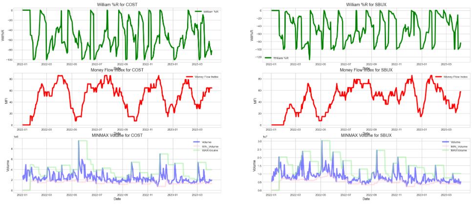
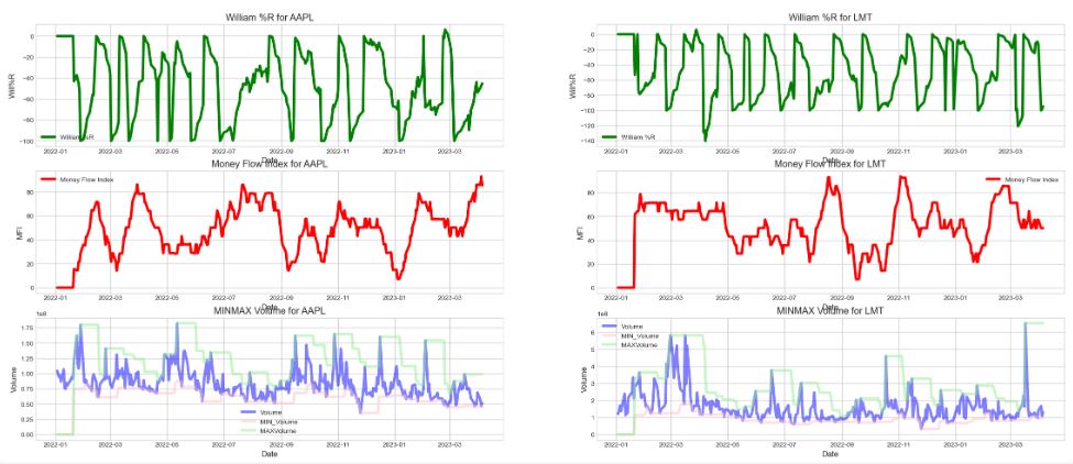
Money Flow Index (MFI)
Money flow is calculated by averaging the high, low and closing prices, and multiplying by the daily volume. Comparing that result with the number for the previous day tells traders whether money flow was positive or negative for the current day. Positive money flow indicates that prices are likely to move higher, while negative money flow suggests prices are about to fall.
Typical Price = (High + Low + Close)/3
Raw Money Flow = Typical Price x Volume
The money flow is divided into positive and negative money flow.
- Positive money flow is calculated by adding the money flow of all the days where the typical price is higher than the previous day’s typical price.
- Negative money flow is calculated by adding the money flow of all the days where the typical price is lower than the previous day’s typical price.
- If typical price is unchanged then that day is discarded.
- Money Flow Ratio = (14-period Positive Money Flow)/(14-period Negative Money Flow)
- Money Flow Index = 100 – 100/(1 + Money Flow Ratio)
def MFI(df):
# typical price
df[‘tp’] = (df[‘High’]+df[‘Low’]+df[‘Close’])/3
#raw money flow
df[‘rmf’] = df[‘tp’] * df[‘Volume’]
# positive and negative money flow
df['pmf'] = np.where(df['tp'] > df['tp'].shift(1), df['tp'], 0)
df['nmf'] = np.where(df['tp'] < df['tp'].shift(1), df['tp'], 0)

# money flow ratio
df['mfr'] = df['pmf'].rolling(window=14,center=False).sum()/df['nmf'].rolling(window=14,center=False).sum()
df['Money_Flow_Index'] = 100 - 100 / (1 + df['mfr'])
for stock in range(len(TechIndicator)):
MFI(TechIndicator[stock])
TechIndicator[stock] = TechIndicator[stock].fillna(0)
TechIndicator[2].tail()
Ichimoku Cloud
- The Ichimoku Cloud is a collection of technical indicators that show support and resistance levels, as well as momentum and trend direction. It does this by taking multiple averages and plotting them on a chart. It also uses these figures to compute a “cloud” that attempts to forecast where the price may find support or resistance in the future.
- The Ichimoku Cloud is composed of five lines or calculations, two of which comprise a cloud where the difference between the two lines is shaded in.
- The lines include a nine-period average, a 26-period average, an average of those two averages, a 52-period average, and a lagging closing price line.
- The cloud is a key part of the indicator. When the price is below the cloud, the trend is down. When the price is above the cloud, the trend is up.
- The above trend signals are strengthened if the cloud is moving in the same direction as the price. For example, during an uptrend, the top of the cloud is moving up, or during a downtrend, the bottom of the cloud is moving down.
- Turning Line = ( Highest High + Lowest Low ) / 2, for the past 9 days
- Standard Line = ( Highest High + Lowest Low ) / 2, for the past 26 days
- Leading Span 1 = ( Standard Line + Turning Line ) / 2, plotted 26 days ahead of today
- Leading Span 2 = ( Highest High + Lowest Low ) / 2, for the past 52 days, plotted 26 days ahead of today
- Cloud = Shaded Area between Span 1 and Span 2
def ichimoku(df):
# Turning Line
period9_high = df[‘High’].rolling(window=9,center=False).max()
period9_low = df[‘Low’].rolling(window=9,center=False).min()
df[‘turning_line’] = (period9_high + period9_low) / 2
# Standard Line
period26_high = df['High'].rolling(window=26,center=False).max()
period26_low = df['Low'].rolling(window=26,center=False).min()
df['standard_line'] = (period26_high + period26_low) / 2

# Leading Span 1
df['ichimoku_span1'] = ((df['turning_line'] + df['standard_line']) / 2).shift(26)

# Leading Span 2
period52_high = df['High'].rolling(window=52,center=False).max()
period52_low = df['Low'].rolling(window=52,center=False).min()
df['ichimoku_span2'] = ((period52_high + period52_low) / 2).shift(26)

# The most current closing price plotted 22 time periods behind (optional)
df['chikou_span'] = df['Close'].shift(-22) # 22 according to investopedia
for stock in range(len(TechIndicator)):
ichimoku(TechIndicator[stock])
TechIndicator[stock] = TechIndicator[stock].fillna(0)
TechIndicator[2].tail()
William %R (WillR)
Williams %R, also known as the Williams Percent Range, is a type of momentum indicator that moves between 0 and -100 and measures overbought and oversold levels. The Williams %R may be used to find entry and exit points in the market. The indicator is very similar to the Stochastic oscillator and is used in the same way.
- Williams %R moves between zero and -100.
- A reading above -20 is overbought.
- A reading below -80 is oversold.
- An overbought or oversold reading doesn’t mean the price will reverse. Overbought simply means the price is near the highs of its recent range, and oversold means the price is in the lower end of its recent range.
- Can be used to generate trade signals when the price and the indicator move out of overbought or oversold territory.
- %R = -100 * ( ( Highest High – Close) / ( Highest High – Lowest Low ) )
def WillR(df):
highest_high = df[‘High’].rolling(window=14,center=False).max()
lowest_low = df[‘Low’].rolling(window=14,center=False).min()
df[‘WillR’] = (-100) * ((highest_high – df[‘Close’]) / (highest_high – lowest_low))
for stock in range(len(TechIndicator)):
WillR(TechIndicator[stock])
TechIndicator[stock] = TechIndicator[stock].fillna(0)
TechIndicator[2].tail()
MINMAX
def MINMAX(df):
df[‘MIN_Volume’] = df[‘Volume’].rolling(window=14,center=False).min()
df[‘MAX_Volume’] = df[‘Volume’].rolling(window=14,center=False).max()
for stock in range(len(TechIndicator)):
MINMAX(TechIndicator[stock])
TechIndicator[stock] = TechIndicator[stock].fillna(0)
TechIndicator[2].tail()
Adaptive Moving Average (KAMA)
Developed by Perry Kaufman, Kaufman’s Adaptive Moving Average (KAMA) is a moving average designed to account for market noise or volatility. KAMA will closely follow prices when the price swings are relatively small and the noise is low. KAMA will adjust when the price swings widen and follow prices from a greater distance. This trend-following indicator can be used to identify the overall trend, time turning points and filter price movements.
def KAMA(price, n=10, pow1=2, pow2=30):
”’ kama indicator ”’
”’ accepts pandas dataframe of prices ”’
absDiffx = abs(price - price.shift(1) )

ER_num = abs( price - price.shift(n) )
ER_den = absDiffx.rolling(window=n,center=False).sum()
ER = ER_num / ER_den

sc = ( ER*(2.0/(pow1+1)-2.0/(pow2+1.0))+2/(pow2+1.0) ) ** 2.0


answer = np.zeros(sc.size)
N = len(answer)
first_value = True

for i in range(N):
    if sc[i] != sc[i]:
        answer[i] = np.nan
    else:
        if first_value:
            answer[i] = price[i]
            first_value = False
        else:
            answer[i] = answer[i-1] + sc[i] * (price[i] - answer[i-1])
return answer
for stock in range(len(TechIndicator)):
TechIndicator[stock][‘KAMA’] = KAMA(TechIndicator[stock][‘Close’])
TechIndicator[stock] = TechIndicator[stock].fillna(0)
TechIndicator[4].tail()
columns2Drop = [’26_ema’, ’12_ema’,’tp’,’rmf’,’pmf’,’nmf’,’mfr’]
for stock in range(len(TechIndicator)):
TechIndicator[stock] = TechIndicator[stock].drop(labels = columns2Drop, axis=1)
TechIndicator[2].head()
Visualization of Technical Indicators
%matplotlib inline
from matplotlib.dates import DateFormatter
Relative Strength Index
fig = plt.figure(figsize=(20,25))
for i in range(8):
ax = plt.subplot(4,2,i+1)
TechIndicator[i][‘mydate’]=pd.to_datetime(TechIndicator[i].index)
ax.plot(TechIndicator[i][‘mydate’], TechIndicator[i][‘RSI_14D’])
ax.set_title(str(TechIndicator[i][‘Label’][0]))
ax.set_xlabel(“Date”)
ax.set_ylabel(“Relative Strength Index”)
plt.xticks(rotation=30)
fig.tight_layout()
plt.savefig(‘vizrsiplot.png’)

Volume Plain
fig = plt.figure(figsize=(20,25))
for i in range(8):
ax = plt.subplot(8,1,i+1)
ax.plot(TechIndicator[i][‘mydate’], TechIndicator[i][‘Volume_plain’], ‘b’)
ax.set_title(str(TechIndicator[i][‘Label’][0]))
ax.set_xlabel(“Date”)
ax.set_ylabel(“Volume”)
plt.xticks(rotation=30)
fig.tight_layout()
plt.savefig(‘vizvolumeplain.png’)
Bollinger Bands
plt.style.use(‘fivethirtyeight’)
fig = plt.figure(figsize=(20,25))
for i in range(8):
ax = plt.subplot(4,2,i+1)
ax.fill_between(TechIndicator[i][‘mydate’], TechIndicator[i][‘BB_Upper_Band’], TechIndicator[i][‘BB_Lower_Band’], color=’grey’, label=”Band Range”)
# Plot Adjust Closing Price and Moving Averages
ax.plot(TechIndicator[i][‘mydate’], TechIndicator[i][‘Close’], color=’red’, lw=2, label=”Close”)
ax.plot(TechIndicator[i][‘mydate’], TechIndicator[i][‘BB_Middle_Band’], color=’black’, lw=2, label=”Middle Band”)
ax.set_title(“Bollinger Bands for ” + str(TechIndicator[i][‘Label’][0]))
ax.legend()
ax.set_xlabel(“Date”)
ax.set_ylabel(“Close Prices”)
plt.xticks(rotation=30)
fig.tight_layout()
plt.savefig(‘vizbollingerbands.png’)

Aroon Oscillator
plt.style.use(‘seaborn-whitegrid’)
fig = plt.figure(figsize=(20,25))
for i in range(8):
ax = plt.subplot(4,2,i+1)
ax.fill(TechIndicator[i][‘mydate’], TechIndicator[i][‘Aroon_Oscillator’],’g’, alpha = 0.5, label = “Aroon Oscillator”)
ax.plot(TechIndicator[i][‘mydate’], TechIndicator[i][‘Close’], ‘r’, label=”Close”)
ax.set_title(“Aroon Oscillator for ” +str(TechIndicator[i][‘Label’][0]))
ax.legend()
ax.set_xlabel(“Date”)
ax.set_ylabel(“Close Prices”)
plt.xticks(rotation=30)
fig.tight_layout()
plt.savefig(‘vizaroonoscillator.png’)
Summary
Price Volume Trend
fig = plt.figure(figsize=(20,25))
for i in range(8):
ax = plt.subplot(8,1,i+1)
ax.plot(TechIndicator[i][‘mydate’], TechIndicator[i][‘PVT’], ‘black’)
ax.set_title(“Price Volume Trend of ” +str(TechIndicator[i][‘Label’][0]))
ax.set_xlabel(“Date”)
ax.set_ylabel(“Price Volume trend”)
plt.xticks(rotation=30)
fig.tight_layout()
plt.savefig(‘vizpricevolumetrend.png’)
Acceleration Band
fig = plt.figure(figsize=(20,25))
for i in range(8):
ax = plt.subplot(4,2,i+1)
ax.fill_between(TechIndicator[i][‘mydate’], TechIndicator[i][‘AB_Upper_Band’], TechIndicator[i][‘AB_Lower_Band’], color=’grey’, label = “Band-Range”)
# Plot Adjust Closing Price and Moving Averages
ax.plot(TechIndicator[i][‘mydate’], TechIndicator[i][‘Close’], color=’red’, lw=2, label = “Close”)
ax.plot(TechIndicator[i][‘mydate’], TechIndicator[i][‘AB_Middle_Band’], color=’black’, lw=2, label=”Middle_Band”)
ax.set_title(“Acceleration Bands for ” + str(TechIndicator[i][‘Label’][0]))
ax.legend()
ax.set_xlabel(“Date”)
ax.set_ylabel(“Close Prices”)
plt.xticks(rotation=30)
fig.tight_layout()
plt.savefig(‘vizaccelerationband.png’)

Stochastic Oscillator
plt.style.use(‘seaborn-whitegrid’)
fig = plt.figure(figsize=(20,25))
for i in range(8):
ax = plt.subplot(4,2,i+1)
ax.plot(TechIndicator[i][‘mydate’], TechIndicator[i][‘STOK’], ‘blue’, label=”%K”)
ax.plot(TechIndicator[i][‘mydate’], TechIndicator[i][‘STOD’], ‘red’, label=”%D”)
ax.plot(TechIndicator[i][‘mydate’], TechIndicator[i][‘Close’], color=’black’, lw=2, label = “Close”)
ax.set_title(“Stochastic Oscillators of ” +str(TechIndicator[i][‘Label’][0]))
ax.legend()
ax.set_xlabel(“Date”)
ax.set_ylabel(“Close Price”)
plt.xticks(rotation=30)
fig.tight_layout()
plt.savefig(‘vizstochasticoscillator.png’)
Chaikin Money Flow
import matplotlib.gridspec as gridspec
fig = plt.figure(figsize=(25,40))
outer = gridspec.GridSpec(4, 2, wspace=0.2, hspace=0.2)
for i in range(8):
inner = gridspec.GridSpecFromSubplotSpec(2, 1,
subplot_spec=outer[i], wspace=0.1, hspace=0.1)
for j in range(2):
    ax = plt.Subplot(fig, inner[j])
    if j==0:
        t = ax.fill(TechIndicator[i]['mydate'], TechIndicator[i]['Chaikin_MF'],'b', alpha = 0.5, label = "Chaikin MF")
        ax.set_title("Chaikin Money Flow for " +str(TechIndicator[i]['Label'][0]))
        t = ax.set_ylabel("Money Flow")
    else:
        t = ax.plot(TechIndicator[i]['mydate'], TechIndicator[i]['Close'], 'r', label="Close")
        t = ax.set_ylabel("Close")
    ax.legend()
    ax.set_xlabel("Date")

    fig.add_subplot(ax)
fig.tight_layout()
plt.savefig(‘vizchaikinmoneyflow.png’)
Parabolic SAR, Rate of Change, Momentum and VWAP
fig = plt.figure(figsize=(20,25))
for i in range(8):
ax = plt.subplot(4,2,i+1)
ax.plot(TechIndicator[i][‘mydate’], TechIndicator[i][‘psar’], ‘blue’, label=”PSAR”, alpha = 0.5)
ax.plot(TechIndicator[i][‘mydate’], TechIndicator[i][‘ROC’], ‘red’, label=”ROC”, alpha = 0.5)
ax.plot(TechIndicator[i][‘mydate’], TechIndicator[i][‘Momentum’], ‘green’, label=”Momentum”, alpha = 0.5)
ax.plot(TechIndicator[i][‘mydate’], TechIndicator[i][‘VWAP’], ‘cyan’, label=”VWAP”, alpha = 0.5)
ax.set_title(“PSAR, ROC, Momentum and VWAP of ” +str(TechIndicator[i][‘Label’][0]))
ax.legend()
ax.set_xlabel(“Date”)
ax.set_ylabel(“Close Price”)
plt.xticks(rotation=30)
fig.tight_layout()
plt.savefig(‘vizpsar.png’)
Commodity Channel Index, Triple Exponential Moving Average On Balance Volume
fig = plt.figure(figsize=(25,80))
outer = gridspec.GridSpec(4, 2, wspace=0.2, hspace=0.2)
for i in range(8):
inner = gridspec.GridSpecFromSubplotSpec(3, 1,
subplot_spec=outer[i], wspace=0.3, hspace=0.3)
for j in range(3):
    ax = plt.Subplot(fig, inner[j])
    if j==0:
        t = ax.plot(TechIndicator[i]['mydate'], TechIndicator[i]['CCI'], 'green', label="CCI")
        t = ax.set_title("CCI for " +str(TechIndicator[i]['Label'][0]))
        t = ax.set_ylabel("Commodity Channel Index")
    elif j == 1:
        t = ax.plot(TechIndicator[i]['mydate'], TechIndicator[i]['TEMA'], 'blue', label="TEMA")
        t = ax.set_title("TEMA for " +str(TechIndicator[i]['Label'][0]))
        t = ax.set_ylabel("TripleExponentiaL MA")
    else:
        t = ax.plot(TechIndicator[i]['mydate'], TechIndicator[i]['OBV'], 'red', label="OBV")
        t = ax.set_title("OBV for " +str(TechIndicator[i]['Label'][0]))
        t = ax.set_ylabel("On Balance Volume")
    ax.legend()

    ax.set_xlabel("Date")

    fig.add_subplot(ax)
fig.tight_layout()
plt.savefig(‘vizccitema.png’)


Normalized Average True Range (NATR)
plt.style.use(‘ggplot’)
fig = plt.figure(figsize=(20,25))
for i in range(8):
ax = plt.subplot(4,2,i+1)
ax.plot(TechIndicator[i][‘mydate’], TechIndicator[i][‘NATR’], ‘red’, label=”NATR”, alpha = 0.5)
ax.plot(TechIndicator[i][‘mydate’], TechIndicator[i][‘Close’], ‘cyan’, label=”Close”, alpha = 0.5)
ax.set_title(“NATR of ” +str(TechIndicator[i][‘Label’][0]))
ax.legend()
ax.set_xlabel(“Date”)
ax.set_ylabel(“Close Price”)
plt.xticks(rotation=30)
fig.tight_layout()
plt.savefig(‘viznatr.png’)

Keltner Channels
fig = plt.figure(figsize=(20,25))
for i in range(8):
ax = plt.subplot(4,2,i+1)
ax.fill_between(TechIndicator[i][‘mydate’], TechIndicator[i][‘Kelch_Upper’], TechIndicator[i][‘Kelch_Down’],
color=’blue’, label = “Band-Range”, alpha = 0.5)
# Plot Adjust Closing Price and Moving Averages
ax.plot(TechIndicator[i][‘mydate’], TechIndicator[i][‘Close’], color=’red’, label = “Close”, alpha = 0.5)
ax.plot(TechIndicator[i][‘mydate’], TechIndicator[i][‘Kelch_Middle’], color=’black’, label=”Middle_Band”, alpha = 0.5)
ax.set_title(“Keltner Channels for ” + str(TechIndicator[i][‘Label’][0]))
ax.legend()
ax.set_xlabel(“Date”)
ax.set_ylabel(“Close Prices”)
plt.xticks(rotation=30)
fig.tight_layout()
plt.savefig(‘vizkeltner.png’)

Average Directional Index
plt.style.use(‘seaborn-whitegrid’)
fig = plt.figure(figsize=(30,25))
for i in range(8):
ax = plt.subplot(4,2,i+1)
ax.plot(TechIndicator[i][‘mydate’], TechIndicator[i][‘plusDI’], ‘green’, label=”+DI”, alpha = 0.5)
ax.plot(TechIndicator[i][‘mydate’], TechIndicator[i][‘minusDI’], ‘cyan’, label=”-DI”, alpha = 0.5)
ax.plot(TechIndicator[i][‘mydate’], TechIndicator[i][‘ADX’], ‘red’, label=”ADX”, alpha = 0.5)
ax.set_title(“Average Directional Index of ” +str(TechIndicator[i][‘Label’][0]))
ax.legend()
ax.set_xlabel(“Date”)
ax.set_ylabel(“Price”)
plt.xticks(rotation=30)
fig.tight_layout()
plt.savefig(‘vizadi.png’)
MACD vs KAMA
plt.style.use(‘seaborn-whitegrid’)
fig = plt.figure(figsize=(20,25))
for i in range(8):
ax = plt.subplot(4,2,i+1)
ax.plot(TechIndicator[i][‘mydate’], TechIndicator[i][‘MACD’], ‘green’, label=”MACD”, alpha = 0.5)
ax.plot(TechIndicator[i][‘mydate’], TechIndicator[i][‘KAMA’], ‘blue’, label=”AMA”, alpha = 0.5)
ax.plot(TechIndicator[i][‘mydate’], TechIndicator[i][‘Close’], ‘red’, label=”Close”, alpha = 0.5)
ax.set_title(“MACD and KAMA of ” +str(TechIndicator[i][‘Label’][0]))
ax.legend()
ax.set_xlabel(“Date”)
ax.set_ylabel(“Price”)
plt.xticks(rotation=30)
fig.tight_layout()
plt.savefig(‘vizmacdkama.png’)
William %R, Money Flow
fig = plt.figure(figsize=(25,50))
outer = gridspec.GridSpec(4, 2, wspace=0.2, hspace=0.2)
for i in range(8):
inner = gridspec.GridSpecFromSubplotSpec(3, 1,
subplot_spec=outer[i], wspace=0.2, hspace=0.2)
for j in range(3):
    ax = plt.Subplot(fig, inner[j])
    if j==0:
        t = ax.plot(TechIndicator[i]['mydate'], TechIndicator[i]['WillR'], 'green', label="William %R")
        t = ax.set_title("William %R for " +str(TechIndicator[i]['Label'][0]))
        t = ax.set_ylabel("Will%R")
    elif j ==1:
        t = ax.plot(TechIndicator[i]['mydate'], TechIndicator[i]['Money_Flow_Index'], 'red', label="Money Flow Index")

        t = ax.set_title("Money Flow Index for " +str(TechIndicator[i]['Label'][0]))
        t = ax.set_ylabel("MFI")
    else:
        t = ax.plot(TechIndicator[i]['mydate'], TechIndicator[i]['Volume'], 'blue', label="Volume", alpha = 0.5)
        t = ax.plot(TechIndicator[i]['mydate'], TechIndicator[i]['MIN_Volume'], 'pink', label="MIN_Volume", alpha = 0.5)
        t = ax.plot(TechIndicator[i]['mydate'], TechIndicator[i]['MAX_Volume'], 'lightgreen', label="MAXVolume",  alpha = 0.5)
        t = ax.set_title("MINMAX Volume for " +str(TechIndicator[i]['Label'][0]))
        t = ax.set_ylabel("Volume")
    ax.legend()
    #ax.set_title("CCI, TEMA, OBV for " +str(techindi2[i]['Label'][0]))
    ax.set_xlabel("Date")

    fig.add_subplot(ax)
fig.tight_layout()
plt.savefig(‘vizwilr.png’)


Ichimoku Cloud
fig = plt.figure(figsize=(20,25)) for i in range(8): ax = plt.subplot(4,2,i+1) ax.fill_between(TechIndicator[i][‘mydate’], TechIndicator[i][‘ichimoku_span1’], TechIndicator[i][‘ichimoku_span2′], color=’blue’, label = “ichimoku cloud”, alpha = 0.5) # Plot Adjust Closing Price and Moving Averages ax.plot(TechIndicator[i][‘mydate’], TechIndicator[i][‘turning_line’], color=’red’, label = “Tenkan-sen”, alpha = 0.4) ax.plot(TechIndicator[i][‘mydate’], TechIndicator[i][‘standard_line’], color=’cyan’, label=”Kijun-sen”, alpha = 0.3) ax.plot(TechIndicator[i][‘mydate’], TechIndicator[i][‘chikou_span’], color=’green’, label=”Chikou-span”, alpha = 0.2) ax.set_title(“Ichimoku for ” + str(TechIndicator[i][‘Label’][0])) ax.legend() ax.set_xlabel(“Date”) ax.set_ylabel(“Prices”) plt.xticks(rotation=30) fig.tight_layout() plt.savefig(‘vizishimoku.png’)

Summary
- In general, technical indicators fit into five categories: trend, mean reversion, relative strength, volume, and momentum.
- Leading indicators attempt to predict where the price is headed while lagging indicators offer a historical report of background conditions that resulted in the current price being where it is.
- Most popular technical indicators include simple moving averages (SMAs), exponential moving averages (EMAs), bollinger bands, stochastics, and on-balance volume (OBV).
- Seven of the best indicators for day trading are:
- On-balance volume (OBV)
- Accumulation/distribution line
- Average directional index
- Aroon oscillator
- Moving average convergence divergence (MACD)
- Relative strength index (RSI)
- Stochastic oscillator
Bottom Line: The most experienced traders are those that have a strong understanding of technical stock indicators, which makes them better equipped to navigate complex and fast-paced financial markets.
Internal Links
- Predicting the JPM Stock Price and Breakouts with Auto ARIMA, FFT, LSTM and Technical Trading Indicators
- The Donchian Channel vs Buy-and-Hold Breakout Trading Systems – $MO Use-Case
- XOM SMA-EMA-RSI Golden Crosses ’22
- The CodeX-Aroon Auto-Trading Approach – the AAPL Use Case
- A TradeSanta’s Quick Guide to Best Swing Trading Indicators
- The Qullamaggie’s OXY Swing Breakouts
- Algorithmic Testing Stock Portfolios to Optimize the Risk/Reward Ratio
- Algorithmic Trading using Monte Carlo Predictions and 62 AI-Assisted Trading Technical Indicators (TTI)
- Predicting Trend Reversal in Algorithmic Trading using Stochastic Oscillator in Python
- Basic Stock Price Analysis in Python
Continue Exploring
- Technical indicators for trading stocks
- Python for stock analysis
- How to Build Stock Technical Indicators with Python
- Mean Reversion Trading Strategy Using Python
Infographic


Embed Socials


Make a one-time donation
Make a monthly donation
Make a yearly donation
Choose an amount
Or enter a custom amount
Your contribution is appreciated.
Your contribution is appreciated.
Your contribution is appreciated.
DonateDonate monthlyDonate yearly
Leave a comment