99% Accurate Breast Cancer Classification using Neural Networks in TensorFlow 2.11.0

Breast cancer (BC) is the second leading cause of death in women all over the world and about 12% of women will suffer from this disease during their lifetime.

Early diagnosis and detection is necessary in order to improve the prognosis of BC.

In principle, available Machine Learning (ML) and Artificial Intelligence (AI) techniques can extract features from images automatically and then perform BC classification.

The recently published review shows that the most successful studies related to AI-driven BC detection applied different types of Neural Network (NN) models to a number of publicly available datasets.

Referring to the earlier AI BC classification experiment and related studies, it appears that one can build and train NN models that accurately predict the probability of BC for individual patients.
Our goal today is to classify whether the BC is benign or malignant by training and testing a NN-classifier. The final goal to establish an accurate NN model to aid radiologists in BC risk estimation.

Workflow

The entire workflow is as follows:

Import Key Libraries
Load Input BC Dataset
Exploratory Data Analysis (EDA)
Data Pre-Processing/Editing/Transformation
Feature Engineering
Train/Test Data Splitting
Build TensorFlow/Keras Model
Compile and Train NN Model
Examine Training/Validation Accuracy
Make Predictions on Test data
Model Classification Report

Prerequisites

We need to install the following libraries:

Numpy
Pandas
Matplotlib
Seaborn
Sklearn
Tensorflow

!pip install –user tensorflow

BC Dataset

In this study, we use the BC Wisconsin (Diagnostic) Dataset to predict whether the BC is benign or malignant.

Model features are computed from a digitized image of a fine needle aspirate (FNA) of a breast mass shown below:

img1 = plt.imread(‘malignant.png’)
img2 = plt.imread(‘benign.png’)

fig, (ax, ax2) = plt.subplots(ncols=2, figsize=(10, 5))
fig.subplots_adjust(wspace=0.5)

ax.imshow(img1)
ax.title.set_text(‘Malignant’)

ax2.imshow(img2)
ax2.title.set_text(‘Benign’)

plt.show()

Images of malignant and benign breast tumors.

Attribute Information:

1) ID number
2) Diagnosis (M = malignant, B = benign)
3-32)

Ten real-valued features are computed for each cell nucleus:

a) radius (mean of distances from center to points on the perimeter)
b) texture (standard deviation of gray-scale values)
c) perimeter
d) area
e) smoothness (local variation in radius lengths)
f) compactness (perimeter^2 / area – 1.0)
g) concavity (severity of concave portions of the contour)
h) concave points (number of concave portions of the contour)
i) symmetry
j) fractal dimension (“coastline approximation” – 1)

All feature values are recorded with 4 significant digits.

Missing attribute values: none

Class distribution: 357 benign, 212 malignant.

TechVidvan NN Model

Let’s set the working directory YOURPATH

import os
os.chdir(‘YOURPATH’) # Set working directory
os. getcwd()

and import libraries for BC classification
import numpy as np
import pandas as pd
import matplotlib.pyplot as plt
import seaborn as sns

Let’s read the input Kaggle data csv file data.csv

df = pd.read_csv(‘data.csv’)

df.head(10)

10 rows × 33 columns

Let’s count the number of rows and columns in dataset:
df.shape

(569, 33)

Let’s look at the pair plot of the input data (selected features)

fig=sns.pairplot(df,hue = ‘diagnosis’, palette= ‘tab10’, vars = [‘radius_mean’, ‘texture_mean’, ‘perimeter_mean’,’area_mean’,’smoothness_mean’])
fig.savefig(“bcdpairplot.png”)

Also, we can count the number of empty values in each column
df.isna().sum()

drop the columns with all the missing values:
df = df.dropna(axis = 1)
df.shape

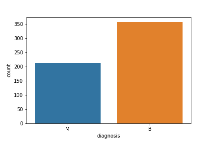
and get the count of the number of Malignant(M) or Benign(B) cells
df[‘diagnosis’].value_counts()

B    357
M    212
Name: diagnosis, dtype: int64

Let’s visualize the count
fig=sns.countplot(df[‘diagnosis’], label = ‘count’)
plt.savefig(“bcdcount.png”)

Let’s look at the data types to see which columns need to be encoded:
df.dtypes

id                           int64
diagnosis                   object
radius_mean                float64
texture_mean               float64
perimeter_mean             float64
area_mean                  float64
smoothness_mean            float64
compactness_mean           float64
concavity_mean             float64
concave points_mean        float64
symmetry_mean              float64
fractal_dimension_mean     float64
radius_se                  float64
texture_se                 float64
perimeter_se               float64
area_se                    float64
smoothness_se              float64
compactness_se             float64
concavity_se               float64
concave points_se          float64
symmetry_se                float64
fractal_dimension_se       float64
radius_worst               float64
texture_worst              float64
perimeter_worst            float64
area_worst                 float64
smoothness_worst           float64
compactness_worst          float64
concavity_worst            float64
concave points_worst       float64
symmetry_worst             float64
fractal_dimension_worst    float64
dtype: object

Rename the diagnosis data to labels:
df = df.rename(columns = {‘diagnosis’ : ‘label’})
print(df.dtypes)

and define the dependent variable that will be predicted (label)
y = df[‘label’].values
print(np.unique(y))

['B' 'M']

Let’s perform encoding categorical data from text(B and M) to integers (0 and 1)
from sklearn.preprocessing import LabelEncoder
labelencoder = LabelEncoder()
Y = labelencoder.fit_transform(y) # M = 1 and B = 0
print(np.unique(Y))

[0 1]

Let’s define the independent variables (features) by dropping label and id

X = df.drop(labels=[‘label’,’id’],axis = 1)

whilst applying MinMaxScaler() to X

from sklearn.preprocessing import MinMaxScaler
scaler = MinMaxScaler()
scaler.fit(X)
X = scaler.transform(X)
print(X)

[[0.52103744 0.0226581  0.54598853 ... 0.91202749 0.59846245 0.41886396]
 [0.64314449 0.27257355 0.61578329 ... 0.63917526 0.23358959 0.22287813]
 [0.60149557 0.3902604  0.59574321 ... 0.83505155 0.40370589 0.21343303]
 ...
 [0.45525108 0.62123774 0.44578813 ... 0.48728522 0.12872068 0.1519087 ]
 [0.64456434 0.66351031 0.66553797 ... 0.91065292 0.49714173 0.45231536]
 [0.03686876 0.50152181 0.02853984 ... 0.         0.25744136 0.10068215]]

Let’s split the data into training and testing datasets (with test_size = 0.25) in order to verify the accuracy after fitting the model
from sklearn.model_selection import train_test_split
x_train,x_test,y_train,y_test = train_test_split(X,Y, test_size = 0.25, random_state=42)
print(‘Shape of training data is: ‘, x_train.shape)
print(‘Shape of testing data is: ‘, x_test.shape)

Shape of training data is:  (426, 30)
Shape of testing data is:  (143, 30)

Let’s invoke TensorFlow with Keras optimizers and create the Sequential model

import tensorflow
from tensorflow.keras.models import Sequential
from tensorflow.keras.layers import Dense, Activation, Dropout
model = Sequential()
model.add(Dense(128, input_dim=30, activation=’relu’))
model.add(Dropout(0.5))
model.add(Dense(64,activation = ‘relu’))
model.add(Dropout(0.5))
model.add(Dense(1))
model.add(Activation(‘sigmoid’))

Let’s compile the NN model

model.compile(loss = ‘binary_crossentropy’, optimizer = ‘adam’ , metrics = [‘accuracy’])
model.summary()

Model: "sequential_4"
_________________________________________________________________
 Layer (type)                Output Shape              Param #   
=================================================================
 dense_12 (Dense)            (None, 128)               3968      
                                                                 
 dropout_8 (Dropout)         (None, 128)               0         
                                                                 
 dense_13 (Dense)            (None, 64)                8256      
                                                                 
 dropout_9 (Dropout)         (None, 64)                0         
                                                                 
 dense_14 (Dense)            (None, 1)                 65        
                                                                 
 activation_4 (Activation)   (None, 1)                 0         
                                                                 
=================================================================
Total params: 12,289
Trainable params: 12,289
Non-trainable params: 0
_________________________________________________________________

let’s fit the model with no early stopping or other callbacks:
history = model.fit(x_train,y_train,verbose = 1,epochs = 100, batch_size = 64,validation_data = (x_test,y_test))

see Appendix A

Let’s plot the training/validation loss vs epochs
loss = history.history[‘loss’]
val_loss = history.history[‘val_loss’]
epochs = range(1,len(loss)+1)
plt.plot(epochs,loss,’y’,label = ‘Training loss’)
plt.plot(epochs,val_loss,’r’,label = ‘Validation loss’)
plt.title(‘TechVidvan NN Training and Validation loss’)
plt.xlabel(‘Epochs’)
plt.ylabel(‘Loss’)
plt.legend()
plt.show()

TechVidvan NN training and validation loss

Let’s plot the training/validation accuracy vs epochs
loss = history.history[‘loss’]
val_loss = history.history[‘val_loss’]
epochs = range(1,len(loss)+1)
plt.plot(epochs,loss,’y’,label = ‘Training loss’)
plt.plot(epochs,val_loss,’r’,label = ‘Validation loss’)
plt.title(‘TechVidvan NN Training and Validation loss’)
plt.xlabel(‘Epochs’)
plt.ylabel(‘Loss’)
plt.legend()
plt.show()

TechVidvan NN training and validation accuracy

Let’s predict the test set results
y_pred = model.predict(x_test)
y_pred = (y_pred > 0.5)

and plot the confusion matrix

from sklearn.metrics import confusion_matrix
cm = confusion_matrix(y_test,y_pred,normalize=’all’)
sns.heatmap(cm, annot = True)

Let’s look at the binary classification report

from sklearn.metrics import classification_report
target_names = [‘B’, ‘M’]
print(classification_report(y_test, y_pred, target_names=target_names))

precision    recall  f1-score   support

           B       0.99      0.98      0.98        89
           M       0.96      0.98      0.97        54

    accuracy                           0.98       143
   macro avg       0.98      0.98      0.98       143
weighted avg       0.98      0.98      0.98       143

Let’s look at other NN model evaluation metrics

from sklearn.metrics import accuracy_score
accuracy_score(y_test, y_pred, normalize=True)

0.9790209790209791

from sklearn.metrics import cohen_kappa_score
cohen_kappa_score(y_test, y_pred)

0.9555302166476625

from sklearn.metrics import hamming_loss
hamming_loss(y_test, y_pred)

0.02097902097902098

from sklearn.metrics import jaccard_score
jaccard_score(y_test, y_pred)

0.9464285714285714

from sklearn.metrics import log_loss
log_loss(y_test, y_pred)

0.7246008977593886

from sklearn.metrics import matthews_corrcoef
matthews_corrcoef(y_test, y_pred)

0.9556352128340201

Optimized Features + SVM/LR + NN

Let’s optimize the NN model by exploring feature engineering and comparing supervised ML (SVM and LR) against Sequential NN described above.

Let’s set the working directory YOURPATH

import os
os.chdir(‘YOURPATH’) # Set working directory
os. getcwd()

import basic libraries

import pandas as pd
import seaborn as sns # for data visualization
import matplotlib.pyplot as plt # for data visualization
%matplotlib inline

and load the input dataset

Data importing and printing
df = pd.read_csv(‘data.csv’)
print(“\nNot processed data. First 10 rows\n”)
df.head(10)

Not processed data. First 10 rows

as a table 10 rows × 33 columns described above.

Let’s install TensorFlow

!pip install –user tensorflow (

tensorflow-2.10.0-cp39-cp39-win_amd64.whl

)

and import the following key libraries

import tensorflow

import os
import numpy as np

from sklearn.preprocessing import StandardScaler

from tensorflow.keras.callbacks import EarlyStopping
from tensorflow.keras.models import Sequential
from tensorflow.keras.layers import Dense

np.random.seed(1337)
os.environ[‘TF_CPP_MIN_LOG_LEVEL’] = ‘3’
pd.set_option(“display.max_column”, 100)
pd.set_option(“display.width”, 1000)

Let’s define the following customized functions

def dataVisualization(data, start=0):
if start == 0:
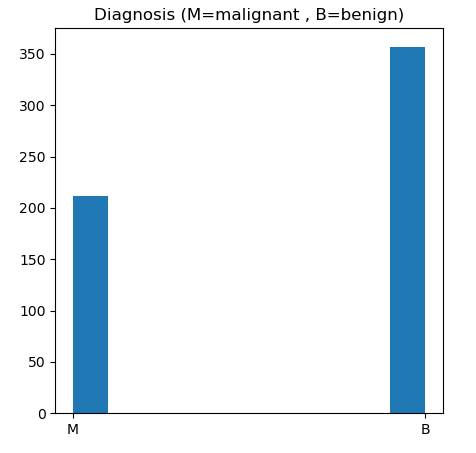
plt.figure(figsize = (5,5))
plt.hist(data[‘diagnosis’])
plt.title(‘Diagnosis (M=malignant , B=benign)’)

    plt.show()
else:
    figures(data, start, start+10)

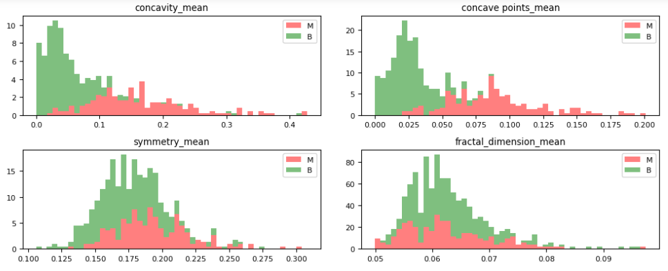
def figures(data, s, e):
plt.rcParams.update({‘font.size’: 8})
fig, axes = plt.subplots(nrows=5, ncols=2, figsize=(10, 10))
axes = axes.ravel()

features = list(data.columns[s:e])

dataM = data[data['diagnosis'] == 'M']
dataB = data[data['diagnosis'] == 'B']

for idx, ax in enumerate(axes):
    ax.figure
    binwidth = (max(data[features[idx]]) - min(data[features[idx]])) / 50
    ax.hist([dataM[features[idx]], dataB[features[idx]]],
            bins=np.arange(min(data[features[idx]]), max(data[features[idx]]) + binwidth, binwidth),
            alpha=0.5, stacked=True, density=True, label=['M', 'B'], color=['r', 'g'])
    ax.legend(loc='upper right')
    ax.set_title(features[idx])

plt.tight_layout()

plt.show()

def dataPreparation(df):
data = df.iloc[:, 1:32]

data['diagnosis'] = data['diagnosis'].map(dict(M=int(1), B=int(0)))
data = data.rename(columns={"diagnosis": "cancer"})
data = data.drop(columns=['perimeter_mean', 'area_mean', 'perimeter_se', 'area_se', 'perimeter_worst', 'area_worst'])

scaler = StandardScaler()

data.iloc[:, 1:] = scaler.fit_transform(data.iloc[:, 1:])

return data

def XYSplit(data):
X = data.iloc[:, 1:]
y = data[‘cancer’]

return X, y

def modelCreate():
callback = EarlyStopping(monitor=’val_loss’, patience=17, restore_best_weights=True)
model = Sequential()

model.add(Dense(50, activation='relu', input_dim=24, kernel_regularizer='l2'))
model.add(Dense(20, activation='relu', kernel_regularizer='l2'))
model.add(Dense(1, activation='sigmoid', name='Output'))

model.compile(loss='binary_crossentropy', optimizer='SGD', metrics=['accuracy'])

return model, callback

def trainingPlot(history):
fig, (ax1, ax2) = plt.subplots(ncols=2, figsize=(10, 5))

ax1.plot(history.history['accuracy'], label='accuracy')
ax1.plot(history.history['val_accuracy'], label='val_accuracy')
ax1.set_xlabel('Epoch')
ax1.set_ylabel('Accuracy')
ax1.set_ylim([0.5, 1])
ax1.legend(loc='lower right')

ax2.plot(history.history['loss'], label='loss')
ax2.plot(history.history['val_loss'], label='val_loss')
ax2.set_xlabel('Epoch')
ax2.set_ylabel('Loss')
ax2.legend(loc='lower right')

plt.show()

def confusionMatrix(cmLR, scoreLR, cmSVM, scoreSVM, cmNN, scoreNN):
fig, (ax1, ax2, ax3) = plt.subplots(ncols=3, figsize=(23, 7))
fig.subplots_adjust(wspace=0.1)

sns.heatmap(cmLR, annot=True, fmt=".3f", linewidths=.7, square=True, cmap='Blues_r', ax=ax1,annot_kws={
            'fontsize': 16,
            'fontweight': 'bold',
            'fontfamily': 'serif'})
ax1.set_ylabel('Actual label',fontsize=16)
ax1.set_xlabel('Predicted label',fontsize=16)
all_sample_title = 'Logistic Regression Score: {0}'.format(round(scoreLR, 5))
ax1.title.set_text(all_sample_title)


cbar = ax1.collections[0].colorbar

cbar.ax1.tick_params(labelsize=16)

sns.heatmap(cmSVM, annot=True, fmt=".3f", linewidths=.7, square=True, cmap='Blues_r', ax=ax2,annot_kws={
            'fontsize': 16,
            'fontweight': 'bold',
            'fontfamily': 'serif'})
ax2.set_ylabel('Actual label',fontsize=16)
ax2.set_xlabel('Predicted label',fontsize=16)
all_sample_title = 'Support Vectore Machine Score: {0}'.format(round(scoreSVM, 5))
ax2.title.set_text(all_sample_title)

sns.heatmap(cmNN, annot=True, fmt=".3f", linewidths=.7, square=True, cmap='Blues_r', ax=ax3,annot_kws={
            'fontsize': 16,
            'fontweight': 'bold',
            'fontfamily': 'serif'})
ax3.set_ylabel('Actual label',fontsize=16)
ax3.set_xlabel('Predicted label',fontsize=16)
all_sample_title = 'Neural Network Score: {0}'.format(round(scoreNN, 5))
ax3.title.set_text(all_sample_title)

plt.show()

Let’s plot the B and M images

img1 = plt.imread(‘malignant.png’)
img2 = plt.imread(‘benign.png’)

fig, (ax, ax2) = plt.subplots(ncols=2, figsize=(10, 5))
fig.subplots_adjust(wspace=0.5)

ax.imshow(img1)
ax.title.set_text(‘Malignant’)

ax2.imshow(img2)
ax2.title.set_text(‘Benign’)

plt.show()

We can check the basic descriptive statistics of both BC outcomes

print(‘Diagnosis = B:’)
df[df[‘diagnosis’] == ‘B’].describe()

Diagnosis = B:

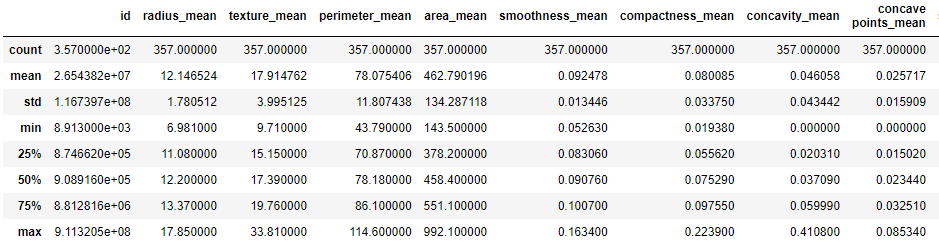
print(‘Diagnosis = M:’)
df[df[‘diagnosis’] == ‘M’].describe()

Diagnosis = M:

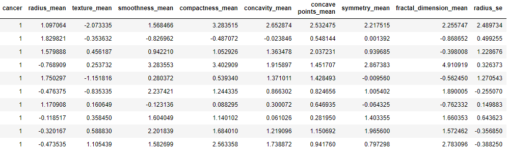
Let’s add more columns
new_col = [‘radius_diff’, ‘texture_diff’, ‘perimeter_diff’, ‘area_diff’,
‘smoothness_diff’, ‘compactness_diff’, ‘concavity_diff’,
‘concave points_diff’, ‘symmetry_diff’, ‘fractal_dimension_diff’]

for i, col in zip(range(len(new_col)), new_col):
df[col] = abs(df.iloc[:, i + 2] – df.iloc[:, i + 22])

df.head(10)

let’s plot the BC M vs B outcomes
dataVisualization(df)

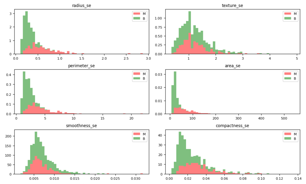
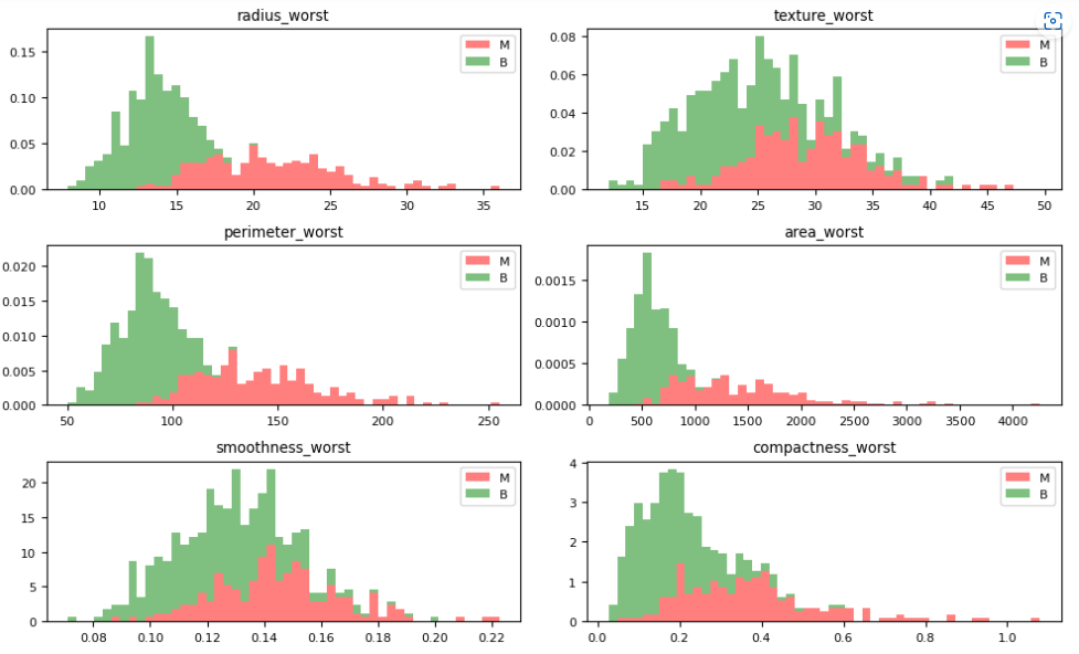
Let’s plot the M vs B histograms of our features

dataVisualization(df, 2)

dataVisualization(df, 12)

dataVisualization(df, 22)

let’s plot the corresponding feature correlation matrices

plt.figure(figsize = (8,8))
corrMatrix = df.iloc[:, 2:12].corr()
sn.heatmap(corrMatrix, annot=True)
plt.show()

plt.figure(figsize = (8,8))
corrMatrix = df.iloc[:, 12:22].corr()
sn.heatmap(corrMatrix, annot=True)
plt.show()

plt.figure(figsize = (8,8))
corrMatrix = df.iloc[:, 22:32].corr()
sn.heatmap(corrMatrix, annot=True)
plt.show()

Data pre-processing:
data = dataPreparation(df)
print(“\nProcessed and standardized data. First 10 rows\n”)
data.head(10)

Processed and standardized data. First 10 rows

Let’s split the data

from sklearn.model_selection import train_test_split

Split into X and y

X, y = XYSplit(data)

Split into train and test

X_train, X_test, y_train, y_test = train_test_split(X, y, test_size=0.25, random_state=7)
print(“The shapes of X_train, X_test, y_train, y_test:”, X_train.shape, X_test.shape, y_train.shape, y_test.shape, ‘\n’)

Let’s compare the Logistic Regression (LR), SVM and NN classifiers

from sklearn.linear_model import LogisticRegression
from sklearn.svm import SVC

Logistic regression training

logreg = LogisticRegression()
logreg.fit(X_train, y_train)

Initialize SVM classifier

SVM = SVC(kernel=’linear’)
SVM.fit(X_train, y_train)

NN model

model, callbacks = modelCreate()
model.summary()

NN training

print(‘\nTraining started…\n’)
history = model.fit(X_train, y_train, epochs=1000, validation_split=0.2, callbacks=[callbacks], verbose=0)
print(f’Training took {len(history.history[“loss”])} epochs’)

Model: "sequential"
_________________________________________________________________
 Layer (type)                Output Shape              Param #   
=================================================================
 dense (Dense)               (None, 50)                1250      
                                                                 
 dense_1 (Dense)             (None, 20)                1020      
                                                                 
 Output (Dense)              (None, 1)                 21        
                                                                 
=================================================================
Total params: 2,291
Trainable params: 2,291
Non-trainable params: 0
_________________________________________________________________

Training started...

Training took 665 epochs

Let’s plot the NN training history
trainingPlot(history)

Let’s make test predictions:

LR testing

scoreLR = logreg.score(X_test, y_test)

SVM testing

scoreSVM = SVM.score(X_test, y_test)

NN testing

scoreNN = model.evaluate(X_test, y_test, verbose=0)[1]

import sklearn

These are LR, SVM, and NN predictions

predictionsLR = logreg.predict(X_test)
cmLR = sklearn.metrics.confusion_matrix(y_test, predictionsLR)
predictionsNN = model.predict(X_test)
predictionsNN = list(map(lambda x: 0 if x < 0.5 else 1, predictionsNN))
cmNN = sklearn.metrics.confusion_matrix(y_test, predictionsNN)

predictionsSVM = SVM.predict(X_test)
cmSVM = sklearn.metrics.confusion_matrix(y_test, predictionsSVM)

And these are the corresponding confusion matrices

confusionMatrix(cmLR, scoreLR, cmSVM, scoreSVM, cmNN, scoreNN)

Let’s look at other model evaluation metrics

print(‘Logistic Regression testing accuracy’, round(scoreLR, 3))

Precision (Accuracy of positive predictions)

precisionLR = cmLR[1,1]/(cmLR[0,1]+cmLR[1,1])
print(‘Precision of Logistic Regression: ‘, round(precisionLR, 3))

Sensitivity=Recall (True Positive Rate)

sensitivityLR = cmLR[1,1]/(cmLR[1,0]+cmLR[1,1])
print(‘Sensitivity/Recall of Logistic Regression: ‘, round(sensitivityLR, 3))

Specificity (True Negative Rate)

specificityLR = cmLR[0,0]/(cmLR[0,0]+cmLR[0,1])
print(‘Specificity of Logistic Regression: ‘, round(specificityLR, 3))

F1-Score (Percent of correct positive predictions)

f1LR = 2(sensitivityLRprecisionLR) / (sensitivityLR+precisionLR)
print(‘F-1 Score of Logistic Regression: ‘, round(specificityLR, 3))

TN FP

FN TP

Logistic Regression testing accuracy 0.972
Precision of Logistic Regression:  1.0
Sensitivity/Recall of Logistic Regression:  0.911
Specificity of Logistic Regression:  1.0
F-1 Score of Logistic Regression:  1.0

print(‘Support Vector Machine testing accuracy’, round(scoreSVM, 3))

Precision (Accuracy of positive predictions)

precisionSVM = cmSVM[1,1]/(cmSVM[0,1]+cmSVM[1,1])
print(‘Precision of Support Vector Machine: ‘, round(precisionSVM, 3))

Sensitivity=Recall (True Positive Rate)

sensitivitySVM = cmSVM[1,1]/(cmSVM[1,0]+cmSVM[1,1])
print(‘Sensitivity/Recall of Support Vector Machine: ‘, round(sensitivitySVM, 3))

Specificity (True Negative Rate)

specificitySVM = cmSVM[0,0]/(cmSVM[0,0]+cmSVM[0,1])
print(‘Specificity of Support Vector Machine: ‘, round(specificitySVM, 3))

F1-Score (Percent of correct positive predictions)

f1SVM = 2(sensitivitySVMprecisionSVM) / (sensitivitySVM+precisionSVM)
print(‘F-1 Score of Support Vector Machine: ‘, round(specificitySVM, 3))

TN FP

FN TP

Support Vector Machine testing accuracy 0.979
Precision of Support Vector Machine:  1.0
Sensitivity/Recall of Support Vector Machine:  0.933
Specificity of Support Vector Machine:  1.0
F-1 Score of Support Vector Machine:  1.0

print(‘Neural Network testing accuracy’, round(scoreNN, 3))

Precision (Accuracy of positive predictions)

precisionNN = cmNN[1,1]/(cmNN[0,1]+cmNN[1,1])
print(‘Precision of Neural Network: ‘, round(precisionNN, 3))

Sensitivity=Recall (True Positive Rate)

sensitivityNN = cmNN[1,1]/(cmNN[1,0]+cmNN[1,1])
print(‘Sensitivity/Recall of Neural Network: ‘, round(sensitivityNN, 3))

Specificity (True Negative Rate)

specificityNN = cmNN[0,0]/(cmNN[0,0]+cmNN[0,1])
print(‘Specificity of Neural Network: ‘, round(specificityNN, 3))

F1-Score (Percent of correct positive predictions)

f1NN = 2(sensitivityNNprecisionNN) / (sensitivityNN+precisionNN)
print(‘F-1 Score of Neural Network: ‘, round(specificityNN, 3))

TN FP

FN TP

Neural Network testing accuracy 0.979
Precision of Neural Network:  1.0
Sensitivity/Recall of Neural Network:  0.933
Specificity of Neural Network:  1.0
F-1 Score of Neural Network:  1.0

Summary

Our NN model accuracy is 99 % on training data and 98% accuracy on validation data.
The NN F1-score is 98% for both classes.
The NN Sensitivity/Recall of Neural Network is 93%.
Confusion matrices of NN and SVM classifiers are identical.
High Pair Correlations: radius_mean – area_mean – perimeter_mean, concavity_mean – compactness_mean, and concave_points_mean – perimeter_mean.

Explore More

The Power of AIHealth: Comparison of 12 ML Breast Cancer Classification Models

Supervised ML/AI Breast Cancer Diagnostics (BCD) – The Power of HealthTech

HealthTech ML/AI Use-Cases

HealthTech ML/AI Q3 ’22 Round-Up

A Comparative Analysis of Breast Cancer ML/AI Binary Classifications

Breast Cancer ML Classification – Logistic Regression vs Gradient Boosting with Hyperparameter Optimization (HPO)

A Comparison of Binary Classifiers for Enhanced ML/AI Breast Cancer Diagnostics – 1. Scikit-Plot

A Comparison of Scikit Learn Algorithms for Breast Cancer Classification – 2. Cross Validation vs Performance

ML/AI Breast Cancer Diagnosis with 98% Confidence

ML/AI Breast Cancer Diagnostics – SciKit-Learn QC

Appendix A

Epoch 1/100
7/7 [==============================] - 0s 17ms/step - loss: 0.6905 - accuracy: 0.5563 - val_loss: 0.6562 - val_accuracy: 0.8252
Epoch 2/100
7/7 [==============================] - 0s 4ms/step - loss: 0.6674 - accuracy: 0.6244 - val_loss: 0.6200 - val_accuracy: 0.8601
Epoch 3/100
7/7 [==============================] - 0s 4ms/step - loss: 0.6362 - accuracy: 0.7324 - val_loss: 0.5793 - val_accuracy: 0.9021
Epoch 4/100
7/7 [==============================] - 0s 4ms/step - loss: 0.5981 - accuracy: 0.7817 - val_loss: 0.5321 - val_accuracy: 0.9161
Epoch 5/100
7/7 [==============================] - 0s 4ms/step - loss: 0.5534 - accuracy: 0.8122 - val_loss: 0.4792 - val_accuracy: 0.9091
Epoch 6/100
7/7 [==============================] - 0s 4ms/step - loss: 0.5106 - accuracy: 0.8216 - val_loss: 0.4238 - val_accuracy: 0.9301
Epoch 7/100
7/7 [==============================] - 0s 4ms/step - loss: 0.4906 - accuracy: 0.8310 - val_loss: 0.3687 - val_accuracy: 0.9441
Epoch 8/100
7/7 [==============================] - 0s 4ms/step - loss: 0.4501 - accuracy: 0.8286 - val_loss: 0.3255 - val_accuracy: 0.9510
Epoch 9/100
7/7 [==============================] - 0s 4ms/step - loss: 0.3961 - accuracy: 0.8779 - val_loss: 0.2818 - val_accuracy: 0.9510
Epoch 10/100
7/7 [==============================] - 0s 4ms/step - loss: 0.3454 - accuracy: 0.8850 - val_loss: 0.2444 - val_accuracy: 0.9510
Epoch 11/100
7/7 [==============================] - 0s 4ms/step - loss: 0.3289 - accuracy: 0.8756 - val_loss: 0.2224 - val_accuracy: 0.9441
Epoch 12/100
7/7 [==============================] - 0s 4ms/step - loss: 0.2757 - accuracy: 0.9155 - val_loss: 0.1917 - val_accuracy: 0.9510
Epoch 13/100
7/7 [==============================] - 0s 3ms/step - loss: 0.2952 - accuracy: 0.8920 - val_loss: 0.1721 - val_accuracy: 0.9441
Epoch 14/100
7/7 [==============================] - 0s 4ms/step - loss: 0.2740 - accuracy: 0.8920 - val_loss: 0.1661 - val_accuracy: 0.9580
Epoch 15/100
7/7 [==============================] - 0s 4ms/step - loss: 0.2697 - accuracy: 0.8991 - val_loss: 0.1570 - val_accuracy: 0.9580
Epoch 16/100
7/7 [==============================] - 0s 3ms/step - loss: 0.2244 - accuracy: 0.9108 - val_loss: 0.1379 - val_accuracy: 0.9441
Epoch 17/100
7/7 [==============================] - 0s 4ms/step - loss: 0.2189 - accuracy: 0.8897 - val_loss: 0.1289 - val_accuracy: 0.9510
Epoch 18/100
7/7 [==============================] - 0s 3ms/step - loss: 0.2353 - accuracy: 0.9085 - val_loss: 0.1317 - val_accuracy: 0.9580
Epoch 19/100
7/7 [==============================] - 0s 4ms/step - loss: 0.1966 - accuracy: 0.9296 - val_loss: 0.1173 - val_accuracy: 0.9720
Epoch 20/100
7/7 [==============================] - 0s 3ms/step - loss: 0.1961 - accuracy: 0.9085 - val_loss: 0.1094 - val_accuracy: 0.9650
Epoch 21/100
7/7 [==============================] - 0s 4ms/step - loss: 0.1926 - accuracy: 0.9061 - val_loss: 0.1066 - val_accuracy: 0.9650
Epoch 22/100
7/7 [==============================] - 0s 3ms/step - loss: 0.1978 - accuracy: 0.9249 - val_loss: 0.1082 - val_accuracy: 0.9720
Epoch 23/100
7/7 [==============================] - 0s 4ms/step - loss: 0.1855 - accuracy: 0.9366 - val_loss: 0.1014 - val_accuracy: 0.9720
Epoch 24/100
7/7 [==============================] - 0s 4ms/step - loss: 0.1641 - accuracy: 0.9507 - val_loss: 0.0922 - val_accuracy: 0.9720
Epoch 25/100
7/7 [==============================] - 0s 4ms/step - loss: 0.1762 - accuracy: 0.9319 - val_loss: 0.0912 - val_accuracy: 0.9790
Epoch 26/100
7/7 [==============================] - 0s 3ms/step - loss: 0.1568 - accuracy: 0.9249 - val_loss: 0.0867 - val_accuracy: 0.9720
Epoch 27/100
7/7 [==============================] - 0s 4ms/step - loss: 0.1681 - accuracy: 0.9319 - val_loss: 0.0850 - val_accuracy: 0.9790
Epoch 28/100
7/7 [==============================] - 0s 4ms/step - loss: 0.1477 - accuracy: 0.9390 - val_loss: 0.0840 - val_accuracy: 0.9790
Epoch 29/100
7/7 [==============================] - 0s 4ms/step - loss: 0.1340 - accuracy: 0.9624 - val_loss: 0.0754 - val_accuracy: 0.9790
Epoch 30/100
7/7 [==============================] - 0s 4ms/step - loss: 0.1570 - accuracy: 0.9437 - val_loss: 0.0815 - val_accuracy: 0.9790
Epoch 31/100
7/7 [==============================] - 0s 4ms/step - loss: 0.1505 - accuracy: 0.9366 - val_loss: 0.0796 - val_accuracy: 0.9790
Epoch 32/100
7/7 [==============================] - 0s 4ms/step - loss: 0.1230 - accuracy: 0.9554 - val_loss: 0.0704 - val_accuracy: 0.9720
Epoch 33/100
7/7 [==============================] - 0s 4ms/step - loss: 0.1404 - accuracy: 0.9484 - val_loss: 0.0700 - val_accuracy: 0.9790
Epoch 34/100
7/7 [==============================] - 0s 4ms/step - loss: 0.1179 - accuracy: 0.9601 - val_loss: 0.0742 - val_accuracy: 0.9790
Epoch 35/100
7/7 [==============================] - 0s 4ms/step - loss: 0.1232 - accuracy: 0.9601 - val_loss: 0.0679 - val_accuracy: 0.9790
Epoch 36/100
7/7 [==============================] - 0s 4ms/step - loss: 0.1211 - accuracy: 0.9624 - val_loss: 0.0655 - val_accuracy: 0.9790
Epoch 37/100
7/7 [==============================] - 0s 5ms/step - loss: 0.1137 - accuracy: 0.9577 - val_loss: 0.0700 - val_accuracy: 0.9790
Epoch 38/100
7/7 [==============================] - 0s 4ms/step - loss: 0.1056 - accuracy: 0.9648 - val_loss: 0.0629 - val_accuracy: 0.9790
Epoch 39/100
7/7 [==============================] - 0s 4ms/step - loss: 0.1183 - accuracy: 0.9531 - val_loss: 0.0647 - val_accuracy: 0.9790
Epoch 40/100
7/7 [==============================] - 0s 4ms/step - loss: 0.1127 - accuracy: 0.9577 - val_loss: 0.0676 - val_accuracy: 0.9790
Epoch 41/100
7/7 [==============================] - 0s 4ms/step - loss: 0.1092 - accuracy: 0.9671 - val_loss: 0.0603 - val_accuracy: 0.9790
Epoch 42/100
7/7 [==============================] - 0s 4ms/step - loss: 0.1150 - accuracy: 0.9577 - val_loss: 0.0616 - val_accuracy: 0.9790
Epoch 43/100
7/7 [==============================] - 0s 6ms/step - loss: 0.0819 - accuracy: 0.9789 - val_loss: 0.0620 - val_accuracy: 0.9790
Epoch 44/100
7/7 [==============================] - 0s 5ms/step - loss: 0.0864 - accuracy: 0.9765 - val_loss: 0.0606 - val_accuracy: 0.9790
Epoch 45/100
7/7 [==============================] - 0s 4ms/step - loss: 0.0922 - accuracy: 0.9671 - val_loss: 0.0625 - val_accuracy: 0.9790
Epoch 46/100
7/7 [==============================] - 0s 4ms/step - loss: 0.0802 - accuracy: 0.9648 - val_loss: 0.0584 - val_accuracy: 0.9790
Epoch 47/100
7/7 [==============================] - 0s 4ms/step - loss: 0.1113 - accuracy: 0.9624 - val_loss: 0.0574 - val_accuracy: 0.9790
Epoch 48/100
7/7 [==============================] - 0s 4ms/step - loss: 0.1092 - accuracy: 0.9554 - val_loss: 0.0578 - val_accuracy: 0.9790
Epoch 49/100
7/7 [==============================] - 0s 4ms/step - loss: 0.0921 - accuracy: 0.9742 - val_loss: 0.0616 - val_accuracy: 0.9790
Epoch 50/100
7/7 [==============================] - 0s 4ms/step - loss: 0.0925 - accuracy: 0.9765 - val_loss: 0.0554 - val_accuracy: 0.9790
Epoch 51/100
7/7 [==============================] - 0s 4ms/step - loss: 0.0931 - accuracy: 0.9648 - val_loss: 0.0561 - val_accuracy: 0.9790
Epoch 52/100
7/7 [==============================] - 0s 4ms/step - loss: 0.1025 - accuracy: 0.9671 - val_loss: 0.0665 - val_accuracy: 0.9790
Epoch 53/100
7/7 [==============================] - 0s 4ms/step - loss: 0.0977 - accuracy: 0.9695 - val_loss: 0.0560 - val_accuracy: 0.9790
Epoch 54/100
7/7 [==============================] - 0s 4ms/step - loss: 0.1016 - accuracy: 0.9671 - val_loss: 0.0558 - val_accuracy: 0.9790
Epoch 55/100
7/7 [==============================] - 0s 4ms/step - loss: 0.0844 - accuracy: 0.9742 - val_loss: 0.0650 - val_accuracy: 0.9790
Epoch 56/100
7/7 [==============================] - 0s 4ms/step - loss: 0.0929 - accuracy: 0.9695 - val_loss: 0.0545 - val_accuracy: 0.9790
Epoch 57/100
7/7 [==============================] - 0s 4ms/step - loss: 0.0744 - accuracy: 0.9812 - val_loss: 0.0539 - val_accuracy: 0.9790
Epoch 58/100
7/7 [==============================] - 0s 4ms/step - loss: 0.0764 - accuracy: 0.9742 - val_loss: 0.0562 - val_accuracy: 0.9790
Epoch 59/100
7/7 [==============================] - 0s 4ms/step - loss: 0.1034 - accuracy: 0.9648 - val_loss: 0.0594 - val_accuracy: 0.9790
Epoch 60/100
7/7 [==============================] - 0s 4ms/step - loss: 0.0789 - accuracy: 0.9695 - val_loss: 0.0529 - val_accuracy: 0.9790
Epoch 61/100
7/7 [==============================] - 0s 3ms/step - loss: 0.0934 - accuracy: 0.9624 - val_loss: 0.0534 - val_accuracy: 0.9790
Epoch 62/100
7/7 [==============================] - 0s 4ms/step - loss: 0.0804 - accuracy: 0.9695 - val_loss: 0.0601 - val_accuracy: 0.9790
Epoch 63/100
7/7 [==============================] - 0s 3ms/step - loss: 0.0832 - accuracy: 0.9695 - val_loss: 0.0565 - val_accuracy: 0.9790
Epoch 64/100
7/7 [==============================] - 0s 3ms/step - loss: 0.0862 - accuracy: 0.9718 - val_loss: 0.0531 - val_accuracy: 0.9790
Epoch 65/100
7/7 [==============================] - 0s 4ms/step - loss: 0.0751 - accuracy: 0.9812 - val_loss: 0.0512 - val_accuracy: 0.9860
Epoch 66/100
7/7 [==============================] - 0s 4ms/step - loss: 0.0724 - accuracy: 0.9812 - val_loss: 0.0530 - val_accuracy: 0.9790
Epoch 67/100
7/7 [==============================] - 0s 4ms/step - loss: 0.0882 - accuracy: 0.9624 - val_loss: 0.0674 - val_accuracy: 0.9720
Epoch 68/100
7/7 [==============================] - 0s 4ms/step - loss: 0.0784 - accuracy: 0.9765 - val_loss: 0.0497 - val_accuracy: 0.9860
Epoch 69/100
7/7 [==============================] - 0s 3ms/step - loss: 0.0732 - accuracy: 0.9789 - val_loss: 0.0531 - val_accuracy: 0.9790
Epoch 70/100
7/7 [==============================] - 0s 3ms/step - loss: 0.0799 - accuracy: 0.9718 - val_loss: 0.0531 - val_accuracy: 0.9790
Epoch 71/100
7/7 [==============================] - 0s 4ms/step - loss: 0.0676 - accuracy: 0.9836 - val_loss: 0.0503 - val_accuracy: 0.9790
Epoch 72/100
7/7 [==============================] - 0s 4ms/step - loss: 0.0647 - accuracy: 0.9789 - val_loss: 0.0522 - val_accuracy: 0.9790
Epoch 73/100
7/7 [==============================] - 0s 4ms/step - loss: 0.0571 - accuracy: 0.9836 - val_loss: 0.0514 - val_accuracy: 0.9790
Epoch 74/100
7/7 [==============================] - 0s 4ms/step - loss: 0.0656 - accuracy: 0.9812 - val_loss: 0.0516 - val_accuracy: 0.9790
Epoch 75/100
7/7 [==============================] - 0s 3ms/step - loss: 0.0640 - accuracy: 0.9742 - val_loss: 0.0566 - val_accuracy: 0.9790
Epoch 76/100
7/7 [==============================] - 0s 3ms/step - loss: 0.0654 - accuracy: 0.9742 - val_loss: 0.0535 - val_accuracy: 0.9790
Epoch 77/100
7/7 [==============================] - 0s 3ms/step - loss: 0.0660 - accuracy: 0.9765 - val_loss: 0.0513 - val_accuracy: 0.9790
Epoch 78/100
7/7 [==============================] - 0s 3ms/step - loss: 0.0576 - accuracy: 0.9812 - val_loss: 0.0516 - val_accuracy: 0.9790
Epoch 79/100
7/7 [==============================] - 0s 4ms/step - loss: 0.0632 - accuracy: 0.9789 - val_loss: 0.0491 - val_accuracy: 0.9790
Epoch 80/100
7/7 [==============================] - 0s 4ms/step - loss: 0.0784 - accuracy: 0.9695 - val_loss: 0.0507 - val_accuracy: 0.9790
Epoch 81/100
7/7 [==============================] - 0s 4ms/step - loss: 0.0629 - accuracy: 0.9812 - val_loss: 0.0585 - val_accuracy: 0.9790
Epoch 82/100
7/7 [==============================] - 0s 4ms/step - loss: 0.0709 - accuracy: 0.9789 - val_loss: 0.0541 - val_accuracy: 0.9790
Epoch 83/100
7/7 [==============================] - 0s 4ms/step - loss: 0.0654 - accuracy: 0.9836 - val_loss: 0.0524 - val_accuracy: 0.9790
Epoch 84/100
7/7 [==============================] - 0s 3ms/step - loss: 0.0678 - accuracy: 0.9812 - val_loss: 0.0510 - val_accuracy: 0.9790
Epoch 85/100
7/7 [==============================] - 0s 4ms/step - loss: 0.0843 - accuracy: 0.9648 - val_loss: 0.0505 - val_accuracy: 0.9790
Epoch 86/100
7/7 [==============================] - 0s 5ms/step - loss: 0.0645 - accuracy: 0.9836 - val_loss: 0.0518 - val_accuracy: 0.9790
Epoch 87/100
7/7 [==============================] - 0s 5ms/step - loss: 0.0567 - accuracy: 0.9859 - val_loss: 0.0529 - val_accuracy: 0.9790
Epoch 88/100
7/7 [==============================] - 0s 5ms/step - loss: 0.0613 - accuracy: 0.9765 - val_loss: 0.0561 - val_accuracy: 0.9790
Epoch 89/100
7/7 [==============================] - 0s 5ms/step - loss: 0.0730 - accuracy: 0.9671 - val_loss: 0.0555 - val_accuracy: 0.9790
Epoch 90/100
7/7 [==============================] - 0s 4ms/step - loss: 0.0498 - accuracy: 0.9859 - val_loss: 0.0535 - val_accuracy: 0.9790
Epoch 91/100
7/7 [==============================] - 0s 7ms/step - loss: 0.0737 - accuracy: 0.9742 - val_loss: 0.0528 - val_accuracy: 0.9790
Epoch 92/100
7/7 [==============================] - 0s 8ms/step - loss: 0.0559 - accuracy: 0.9859 - val_loss: 0.0498 - val_accuracy: 0.9790
Epoch 93/100
7/7 [==============================] - 0s 7ms/step - loss: 0.0574 - accuracy: 0.9836 - val_loss: 0.0535 - val_accuracy: 0.9790
Epoch 94/100
7/7 [==============================] - 0s 6ms/step - loss: 0.0461 - accuracy: 0.9883 - val_loss: 0.0546 - val_accuracy: 0.9790
Epoch 95/100
7/7 [==============================] - 0s 8ms/step - loss: 0.0527 - accuracy: 0.9836 - val_loss: 0.0523 - val_accuracy: 0.9790
Epoch 96/100
7/7 [==============================] - 0s 6ms/step - loss: 0.0630 - accuracy: 0.9789 - val_loss: 0.0519 - val_accuracy: 0.9790
Epoch 97/100
7/7 [==============================] - 0s 7ms/step - loss: 0.0649 - accuracy: 0.9718 - val_loss: 0.0516 - val_accuracy: 0.9790
Epoch 98/100
7/7 [==============================] - 0s 9ms/step - loss: 0.0642 - accuracy: 0.9718 - val_loss: 0.0502 - val_accuracy: 0.9860
Epoch 99/100
7/7 [==============================] - 0s 4ms/step - loss: 0.0622 - accuracy: 0.9812 - val_loss: 0.0544 - val_accuracy: 0.9790
Epoch 100/100
7/7 [==============================] - 0s 4ms/step - loss: 0.0695 - accuracy: 0.9765 - val_loss: 0.0535 - val_accuracy: 0.9790

Make a one-time donation

Make a monthly donation

Make a yearly donation

Choose an amount

$5.00

$15.00

$100.00

$5.00

$15.00

$100.00

$5.00

$15.00

$100.00

Or enter a custom amount

Your contribution is appreciated.

Donate Donate monthly Donate yearly

7 responses to “99% Accurate Breast Cancer Classification using Neural Networks in TensorFlow 2.11.0”

Hairstyles says:

23rd Dec 2022 at 11:17 am

whoah this blog is great i love reading your articles. Keep up the good work! You know, lots of people are hunting around for this information, you could aid them greatly.

LikeLiked by 1 person

website says:

3rd Jan 2023 at 1:39 pm

I have read several good stuff here. Certainly worth bookmarking for revisiting. I wonder how much effort you put to create such a fantastic informative web site.

LikeLike

Blake Pultz says:

17th Feb 2023 at 8:34 pm

I like what you guys are up too. Such clever work and reporting! Keep up the superb works guys I have incorporated you guys to my blogroll. I think it will improve the value of my site 🙂

LikeLiked by 1 person

droppin says:

19th Feb 2023 at 12:26 am

As I web-site possessor I believe the content material here is rattling magnificent , appreciate it for your hard work. You should keep it up forever! Best of luck.

LikeLike

https://www.instructables.com says:

24th Feb 2023 at 3:13 pm

https://community.datastax.com/users/7690/masterscom.html
Everything is very open with a precise description of the challenges.
It was definitely informative. Your website is extremely helpful.
Many thanks for sharing!

LikeLike

https://www.zintro.com/ says:

27th Feb 2023 at 2:01 pm

https://www.empowher.com/users/masterscom
Just wish to say your article is as amazing. The clearness on your
submit is simply spectacular and i can assume you’re knowledgeable on this
subject. Well together with your permission allow me to seize your RSS feed to stay updated with drawing close post.
Thanks 1,000,000 and please carry on the rewarding work.

LikeLike

is.gd says:

4th Mar 2023 at 7:05 pm

https://tinyurl.com/mtx7vetm
I am not sure where you are getting your info, but good topic.
I needs to spend some time learning more or understanding
more. Thanks for fantastic information I was looking for this info for my
mission.

LikeLike

99% Accurate Breast Cancer Classification using Neural Networks in TensorFlow 2.11.0

Workflow

Prerequisites

BC Dataset

TechVidvan NN Model

Let’s look at the pair plot of the input data (selected features)

Optimized Features + SVM/LR + NN

Split into X and y

Split into train and test

Logistic regression training

Initialize SVM classifier

NN model

NN training

LR testing

SVM testing

NN testing

These are LR, SVM, and NN predictions

And these are the corresponding confusion matrices

Precision (Accuracy of positive predictions)

Sensitivity=Recall (True Positive Rate)

Specificity (True Negative Rate)

F1-Score (Percent of correct positive predictions)

TN FP

FN TP

Precision (Accuracy of positive predictions)

Sensitivity=Recall (True Positive Rate)

Specificity (True Negative Rate)

F1-Score (Percent of correct positive predictions)

TN FP

FN TP

Precision (Accuracy of positive predictions)

Sensitivity=Recall (True Positive Rate)

Specificity (True Negative Rate)

F1-Score (Percent of correct positive predictions)

TN FP

FN TP

Summary

Explore More

Appendix A

Make a one-time donation

Make a monthly donation

Make a yearly donation

Share this:

Like this:

7 responses to “99% Accurate Breast Cancer Classification using Neural Networks in TensorFlow 2.11.0”

Leave a Reply Cancel reply