ML/AI Breast Cancer Diagnosis with 98% Confidence

Featured Photo by Andrew Neel

This healthtech use-case study is dedicated to #BreastCancerAwarenessMonth2022 #breastcancer #BreastCancerDay @Breastcancerorg @BCAction @BCRFcure @NBCF @LivingBeyondBC @breastcancer @TheBreastCancer @thepinkribbon @BreastCancerNow.

The WHO reports that cancer, such as breast, cervical, ovarian, lung and prostate cancer, has accounted for over 10 million deaths in 2022. Breast cancer (BC) is one of the most prevailing cancers among women worldwide.

Recently, Machine Learning (ML) techniques have been employed in healthtech to help diagnose BC at an early stage.

The goal of this study is to demonstrate the importance of hyperparameter optimization (HPO) for enhancing ML prediction accuracy. Specifically, we will focus on the Random Forest Classifier (RFC) as an ensemble of decision trees. RFC is a supervised ML algorithm that has been applied successfully to the BC binary classification. 

We use the publicly available BC dataset from the University of Wisconsin Hospitals, Madison, Wisconsin, USA. 

Let’s open the Jupyter IDE Notebook to implement the following ML workflow:

• Importing relevant libraries
• Import and explore input data
• Data preparation/transformation for ML
• Training/testing RFC model
• GridSearchCV HPO
• Scikit Plot QC analysis

Contents:

1. ML Pipeline
2. QC Analysis
3. Summary
4. Explore More
5. Bottom Line

ML Pipeline

We begin by setting the working directory YOURPATH

import os
os.chdir(‘YOURPATH’)
os. getcwd()

and importing the following libraries

!pip install opencv-python

import cv2
import tensorflow
from tensorflow.keras.applications import ResNet50,MobileNet, DenseNet201, InceptionV3, NASNetLarge, InceptionResNetV2, NASNetMobile
opt = tensorflow.keras.optimizers.Adam(learning_rate=0.1)

import json
import math
import os

from PIL import Image
import numpy as np
from keras import layers
from keras.callbacks import Callback, ModelCheckpoint, ReduceLROnPlateau, TensorBoard
from keras.preprocessing.image import ImageDataGenerator
from keras.utils.np_utils import to_categorical
from keras.models import Sequential
import matplotlib.pyplot as plt
import pandas as pd
from sklearn.model_selection import train_test_split
from sklearn.metrics import cohen_kappa_score, accuracy_score
import scipy
from tqdm import tqdm
import tensorflow as tf
from keras import backend as K
import gc

import pandas as pd
from functools import partial
from sklearn import metrics
from collections import Counter

from sklearn.preprocessing import LabelEncoder

from sklearn.ensemble import RandomForestClassifier

from sklearn.metrics import accuracy_score

from sklearn.model_selection import GridSearchCV

from sklearn.model_selection import train_test_split

!pip install scikit-plot

import scikitplot as skplt

import sklearn
from sklearn.datasets import load_digits, load_boston, load_breast_cancer
from sklearn.model_selection import train_test_split

from sklearn.ensemble import RandomForestClassifier, RandomForestRegressor, GradientBoostingClassifier, ExtraTreesClassifier
from sklearn.linear_model import LinearRegression, LogisticRegression
from sklearn.cluster import KMeans
from sklearn.decomposition import PCA

import matplotlib.pyplot as plt

import sys
import warnings
warnings.filterwarnings(“ignore”)

print(“Scikit Plot Version : “, skplt.version)
print(“Scikit Learn Version : “, sklearn.version)
print(“Python Version : “, sys.version)

import json
import itertools

%matplotlib inline

Scikit Plot Version :  0.3.7
Scikit Learn Version :  1.0.2
Python Version :  3.9.13 (main, Aug 25 2022, 23:51:50) [MSC v.1916 64 bit (AMD64)]

Let’s read the input BC dataset

df = pd.read_csv( “data.csv”)

and checks the structure of this table

df.head()

df.shape

(569, 33)

Let’s define the target column

y = df.loc[:,”diagnosis”].values

and the feature column

X = df.drop([“diagnosis”,”id”,”Unnamed: 32″],axis=1).values

Let’s apply LabelEncoder to the target variable

le = LabelEncoder()

y = le.fit_transform(y)

Let’s split the input dataset without scaling our features

X_train,X_test,y_train,y_test=train_test_split(X, y,
stratify=y,
random_state=0)

We are ready to apply RFC to the train data

rf = RandomForestClassifier(random_state = 0)

rf.fit(X_train, y_train)

RandomForestClassifier(random_state=0)

and perform train/test data predictions

y_train_pred = rf.predict(X_train)
y_test_pred = rf.predict(X_test)

while evaluating their accuracy scores

rf_train = accuracy_score(y_train, y_train_pred)
rf_test = accuracy_score(y_test, y_test_pred)

print(f’Random forest train/test accuracies: {rf_train: .3f}/{rf_test:.3f}’)

Random forest train/test accuracies:  1.000/0.958

It is time to apply GridSearchCV to RFC

rf = RandomForestClassifier(random_state = 42)

by setting the following HPO parameters

parameters = {‘max_depth’:[5,10,20],’n_estimators’:[i for i in range(10, 100, 10)],’min_samples_leaf’:[i for i in range(1, 10)],’criterion’ :[‘gini’, ‘entropy’],’max_features’: [‘auto’, ‘sqrt’, ‘log2’]}

Let’s apply the HPO operator

clf = GridSearchCV(rf, parameters, n_jobs= -1)

to the train data

clf.fit(X_train, y_train)

GridSearchCV(estimator=RandomForestClassifier(random_state=42), n_jobs=-1,
             param_grid={'criterion': ['gini', 'entropy'],
                         'max_depth': [5, 10, 20],
                         'max_features': ['auto', 'sqrt', 'log2'],
                         'min_samples_leaf': [1, 2, 3, 4, 5, 6, 7, 8, 9],
                         'n_estimators': [10, 20, 30, 40, 50, 60, 70, 80, 90]})

This yields the best HPO parameters

print(clf.best_params_)

{'criterion': 'entropy', 'max_depth': 10, 'max_features': 'log2', 'min_samples_leaf': 2, 'n_estimators': 20}

Let’s perform our predictions

y_train_pred=clf.predict(X_train)
y_test_pred=clf.predict(X_test)
rf_train = accuracy_score(y_train, y_train_pred)
rf_test = accuracy_score(y_test, y_test_pred)
print(f’Random forest train/test accuracies: {rf_train: .3f}/{rf_test:.3f}’)

Random forest train/test accuracies:  0.991/0.958

QC Analysis

Let’s invoke Scikit Plot to assess the above ML results:

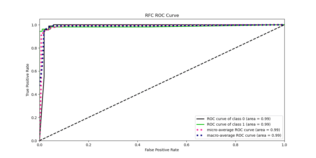
• ROC curve

Clearly, we want a value on this curve close to (0,1) as this would imply a perfect model; 100% specificity and sensitivity. 

• Precision-Recall Curve

• KS Statistic Plot

Tt helps us to understand how well our predictive model is able to discriminate between two classes.

• Cumulative Gains Curve

RFC is the best classifier because

• the optimal classifier will score positives and negatives s.t. there’s a clear separation between them
• in such a case the gain chart will always go up until it reaches 1, and then go left

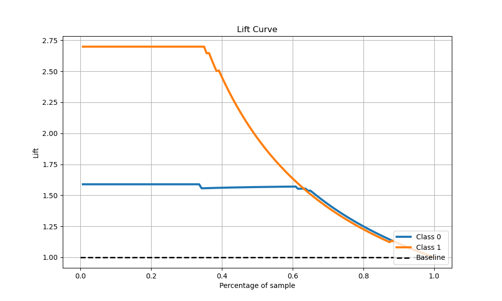
• Lift Curve

The Lift of 2.7 for top two deciles, means that when selecting 20% of the records based on the model, one can expect 2.7 times the total number of class 0 found by randomly selecting 20%-of-file without a model.

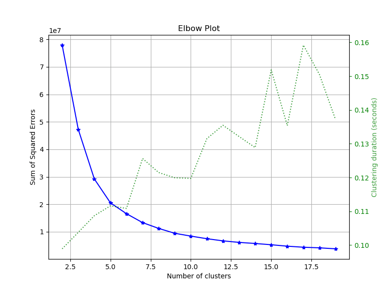
• Elbow Plot

The optimal number of clusters is 5.

• Silhouette Analysis

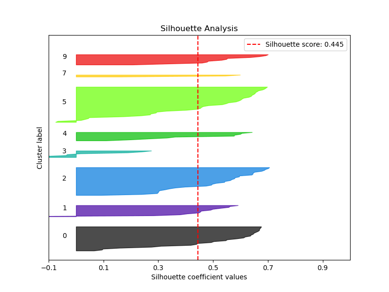
The Silhouette score is 0.445

• PCA Component Explained Variances

We have 0.982 explained variance ratio for first 1 components

• PCA 2-D Projection

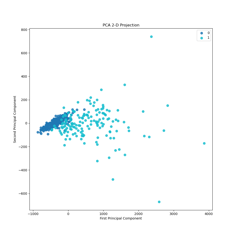
The separation boundary between two classes is clearly visible.

Summary

• This ML workflow predicts whether the BC is benign or malignant (binary classification) using the input BC Wisconsin (diagnostic) dataset
• We have tested the HPO+RFC algorithm GridSearchCV+RandomForestClassifier
• Random forest train/test accuracies: 0.991/0.958
• The ROC area for both classes is 0.99
• The Precision-Recall area for both classes is 0.98
• KS statistic: 0.951 at 0.592
• Both the Cumulative Gains/Lift Curve and the PCA 2-D Projection show good separation of two classes
• The optimal number of clusters is 5 with the Silhouette score of 0.445
• We have 0.982 explained variance ratio for first 1 components.

These results demonstrate the importance of combining HPO and RFC into a single ML framework to optimize the advantages of each. The proposed workflow achieves the best accuracy with the lowest error rate in analyzing the data. It confirms the earlier observations that RFC can provide better accuracy than decision trees since it overcomes the data overfitting problem.

Explore More

• Supervised ML/AI Breast Cancer Diagnostics (BCD) – The Power of HealthTech
• HealthTech ML/AI Use-Cases
• HealthTech ML/AI Q3 ’22 Round-Up
• A Comparative Analysis of Breast Cancer ML/AI Binary Classifications
• Breast Cancer ML Classification – Logistic Regression vs Gradient Boosting with Hyperparameter Optimization (HPO)

Bottom Line