
According to WHO, Breast Cancer (BC) is the leading cause of death among women worldwide. The present study optimizes the use of supervised Machine Learning (ML) algorithms for detecting, analyzing, and classifying BC.
Following previous BC ML/AI case studies (cf. Read More), our objective is to compare Logistic Regression (LR) against Gradient Boosting (GB) Classifier within the Hyperparameter Optimization (HPO) loop given by GridSearchCV.
We use the publicly available BC dataset from the University of Wisconsin Hospitals, Madison, Wisconsin, USA.
Let’s open the Jupyter IDE Notebook
and begin our project by setting the working directory YOURPATH
import os
os.chdir(‘YOURPATH’)
os. getcwd()
and importing the key libraries
import matplotlib.pyplot as plt
import seaborn as sns
import pandas as pd
import numpy as np
from collections import OrderedDict
from sklearn import datasets
from sklearn.preprocessing import label_binarize, LabelBinarizer
from sklearn.model_selection import train_test_split, GridSearchCV
from sklearn.linear_model import LogisticRegression
from sklearn.ensemble import GradientBoostingClassifier
from sklearn.metrics import precision_recall_curve
from sklearn.metrics import classification_report
from sklearn.metrics import roc_curve, auc
DISPLAY_PRECISION = 4
pd.set_option(“display.precision”, DISPLAY_PRECISION)
Let’s load the BC dataset and print its detailed description
dat = datasets.load_breast_cancer()
print(dat.DESCR)
.. _breast_cancer_dataset:

Breast cancer wisconsin (diagnostic) dataset
--------------------------------------------

**Data Set Characteristics:**

    :Number of Instances: 569

    :Number of Attributes: 30 numeric, predictive attributes and the class

    :Attribute Information:
        - radius (mean of distances from center to points on the perimeter)
        - texture (standard deviation of gray-scale values)
        - perimeter
        - area
        - smoothness (local variation in radius lengths)
        - compactness (perimeter^2 / area - 1.0)
        - concavity (severity of concave portions of the contour)
        - concave points (number of concave portions of the contour)
        - symmetry
        - fractal dimension ("coastline approximation" - 1)

        The mean, standard error, and "worst" or largest (mean of the three
        worst/largest values) of these features were computed for each image,
        resulting in 30 features.  For instance, field 0 is Mean Radius, field
        10 is Radius SE, field 20 is Worst Radius.

        - class:
                - WDBC-Malignant
                - WDBC-Benign

    :Summary Statistics:

    ===================================== ====== ======
                                           Min    Max
    ===================================== ====== ======
    radius (mean):                        6.981  28.11
    texture (mean):                       9.71   39.28
    perimeter (mean):                     43.79  188.5
    area (mean):                          143.5  2501.0
    smoothness (mean):                    0.053  0.163
    compactness (mean):                   0.019  0.345
    concavity (mean):                     0.0    0.427
    concave points (mean):                0.0    0.201
    symmetry (mean):                      0.106  0.304
    fractal dimension (mean):             0.05   0.097
    radius (standard error):              0.112  2.873
    texture (standard error):             0.36   4.885
    perimeter (standard error):           0.757  21.98
    area (standard error):                6.802  542.2
    smoothness (standard error):          0.002  0.031
    compactness (standard error):         0.002  0.135
    concavity (standard error):           0.0    0.396
    concave points (standard error):      0.0    0.053
    symmetry (standard error):            0.008  0.079
    fractal dimension (standard error):   0.001  0.03
    radius (worst):                       7.93   36.04
    texture (worst):                      12.02  49.54
    perimeter (worst):                    50.41  251.2
    area (worst):                         185.2  4254.0
    smoothness (worst):                   0.071  0.223
    compactness (worst):                  0.027  1.058
    concavity (worst):                    0.0    1.252
    concave points (worst):               0.0    0.291
    symmetry (worst):                     0.156  0.664
    fractal dimension (worst):            0.055  0.208
    ===================================== ====== ======

    :Missing Attribute Values: None

    :Class Distribution: 212 - Malignant, 357 - Benign

    :Creator:  Dr. William H. Wolberg, W. Nick Street, Olvi L. Mangasarian

    :Donor: Nick Street

    :Date: November, 1995

This is a copy of UCI ML Breast Cancer Wisconsin (Diagnostic) datasets.
https://goo.gl/U2Uwz2

Features are computed from a digitized image of a fine needle
aspirate (FNA) of a breast mass.  They describe
characteristics of the cell nuclei present in the image.

Separating plane described above was obtained using
Multisurface Method-Tree (MSM-T) [K. P. Bennett, "Decision Tree
Construction Via Linear Programming." Proceedings of the 4th
Midwest Artificial Intelligence and Cognitive Science Society,
pp. 97-101, 1992], a classification method which uses linear
programming to construct a decision tree.  Relevant features
were selected using an exhaustive search in the space of 1-4
features and 1-3 separating planes.

The actual linear program used to obtain the separating plane
in the 3-dimensional space is that described in:
[K. P. Bennett and O. L. Mangasarian: "Robust Linear
Programming Discrimination of Two Linearly Inseparable Sets",
Optimization Methods and Software 1, 1992, 23-34].

This database is also available through the UW CS ftp server:

ftp ftp.cs.wisc.edu
cd math-prog/cpo-dataset/machine-learn/WDBC/

.. topic:: References

   - W.N. Street, W.H. Wolberg and O.L. Mangasarian. Nuclear feature extraction
     for breast tumor diagnosis. IS&T/SPIE 1993 International Symposium on
     Electronic Imaging: Science and Technology, volume 1905, pages 861-870,
     San Jose, CA, 1993.
   - O.L. Mangasarian, W.N. Street and W.H. Wolberg. Breast cancer diagnosis and
     prognosis via linear programming. Operations Research, 43(4), pages 570-577,
     July-August 1995.
   - W.H. Wolberg, W.N. Street, and O.L. Mangasarian. Machine learning techniques
     to diagnose breast cancer from fine-needle aspirates. Cancer Letters 77 (1994)
     163-171.
Let’s look at the basic structure of our input data
print(“The sklearn breast cancer dataset keys:”)
print(dat.keys()) # dict_keys([‘target_names’, ‘target’, ‘feature_names’, ‘data’, ‘DESCR’])
print(“—“)
li_classes = [dat.target_names[1], dat.target_names[0]]
li_target = [1 if x==0 else 0 for x in list(dat.target)]
li_ftrs = list(dat.feature_names)
print(“There are 2 target classes:”)
print(“li_classes”, li_classes)
print(“—“)
print(“Target class distribution from a total of %d target values:” % len(li_target))
print(pd.Series(li_target).value_counts())
print(“—“)
df_all = pd.DataFrame(dat.data[:,:], columns=li_ftrs)
print(“Describe dataframe, first 6 columns:”)
print(df_all.iloc[:,:6].describe().to_string())
The sklearn breast cancer dataset keys:
dict_keys(['data', 'target', 'frame', 'target_names', 'DESCR', 'feature_names', 'filename', 'data_module'])
---
There are 2 target classes:
li_classes ['benign', 'malignant']
---
Target class distribution from a total of 569 target values:
0    357
1    212
dtype: int64
---
Describe dataframe, first 6 columns:
       mean radius  mean texture  mean perimeter  mean area  mean smoothness  mean compactness
count     569.0000      569.0000         569.000   569.0000         569.0000          569.0000
mean       14.1273       19.2896          91.969   654.8891           0.0964            0.1043
std         3.5240        4.3010          24.299   351.9141           0.0141            0.0528
min         6.9810        9.7100          43.790   143.5000           0.0526            0.0194
25%        11.7000       16.1700          75.170   420.3000           0.0864            0.0649
50%        13.3700       18.8400          86.240   551.1000           0.0959            0.0926
75%        15.7800       21.8000         104.100   782.7000           0.1053            0.1304
max        28.1100       39.2800         188.500  2501.0000           0.1634            0.3454
Let’s perform test/train data splitting with test_size=0.3
TEST_SIZE_RATIO = 0.3
Setup X and y:
X = df_all
y = pd.Series(li_target)
X_train_0, X_test_0, y_train, y_test = train_test_split(X, y, test_size=TEST_SIZE_RATIO, random_state=0)
print(“X_train_0.shape, y_train.shape”, X_train_0.shape, y_train.shape)
print(“X_test_0.shape, y_test.shape”, X_test_0.shape, y_test.shape)
X_train_0.shape, y_train.shape (398, 30) (398,)
X_test_0.shape, y_test.shape (171, 30) (171,)
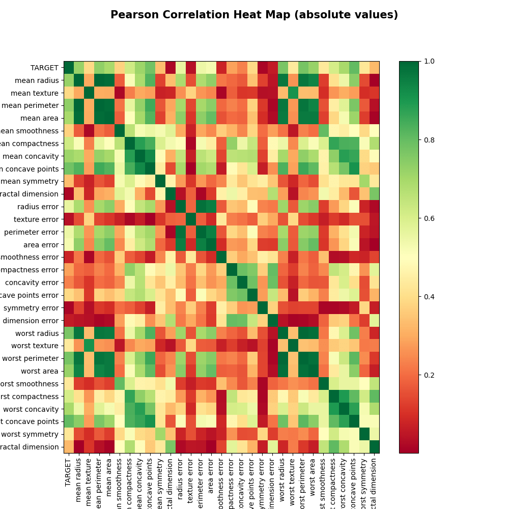
Let’s build the correlation matrix for the train data using the function
def correlation_matrix(y, X, is_plot=False):
# Calculate and plot the correlation symmetrical matrix
# Return:
# yX – concatenated data
# yX_corr – correlation matrix, pearson correlation of values from -1 to +1
# yX_abs_corr – correlation matrix, absolute values
yX = pd.concat([y, X], axis=1)
yX = yX.rename(columns={0: ‘TARGET’}) # rename first column
print(“Function correlation_matrix: X.shape, y.shape, yX.shape:”, X.shape, y.shape, yX.shape)
print()
# Get feature correlations and transform to dataframe
yX_corr = yX.corr(method=’pearson’)
# Convert to abolute values
yX_abs_corr = np.abs(yX_corr)
if is_plot:
plt.figure(figsize=(10, 10))
plt.imshow(yX_abs_corr, cmap=’RdYlGn’, interpolation=’none’, aspect=’auto’)
plt.colorbar()
plt.xticks(range(len(yX_abs_corr)), yX_abs_corr.columns, rotation=’vertical’)
plt.yticks(range(len(yX_abs_corr)), yX_abs_corr.columns);
plt.suptitle(‘Pearson Correlation Heat Map (absolute values)’, fontsize=15, fontweight=’bold’)
#plt.show()
plt.savefig(‘corrmatrixafter.png’)
return yX, yX_corr, yX_abs_corr
Let’s call this function
yX, yX_corr, yX_abs_corr = correlation_matrix(y_train, X_train_0, is_plot=True)
Function correlation_matrix: X.shape, y.shape, yX.shape: (398, 30) (398,) (398, 31)
Let’s select the BC model features within the range (0.1, 0.8)
CORRELATION_MIN = 0.1
Sort features by their Pearson correlation with the target value
s_corr_target = yX_abs_corr[‘TARGET’]
s_corr_target_sort = s_corr_target.sort_values(ascending=False)
Only use features with a minimum Pearson correlation with the target of 0.1
s_low_correlation_ftrs = s_corr_target_sort[s_corr_target_sort <= CORRELATION_MIN]
print(“Removed %d low correlation features:” % len(s_low_correlation_ftrs))
for i,v in enumerate(s_low_correlation_ftrs):
print(i,np.round(v, DISPLAY_PRECISION), s_low_correlation_ftrs.index[i])
print(“—“)
s_corr_target_sort = s_corr_target_sort[s_corr_target_sort > CORRELATION_MIN]
print(“Remaining %d feature correlations:” % (len(s_corr_target_sort)-1))
for i,v in enumerate(s_corr_target_sort):
ftr = s_corr_target_sort.index[i]
if ftr == ‘TARGET’:
continue
print(i,np.round(v, DISPLAY_PRECISION), ftr)
Removed 5 low correlation features:
0 0.0778 smoothness error
1 0.0622 fractal dimension error
2 0.0373 texture error
3 0.0187 mean fractal dimension
4 0.0154 symmetry error
---
Remaining 25 feature correlations:
1 0.8024 worst concave points
2 0.7794 mean concave points
3 0.7723 worst perimeter
4 0.7661 worst radius
5 0.7318 mean perimeter
6 0.7194 worst area
7 0.719 mean radius
8 0.7111 mean concavity
9 0.6947 worst concavity
10 0.6932 mean area
11 0.6196 mean compactness
12 0.6062 worst compactness
13 0.5574 radius error
14 0.5465 perimeter error
15 0.5264 area error
16 0.4347 worst texture
17 0.4324 worst smoothness
18 0.4255 worst symmetry
19 0.3902 concave points error
20 0.3883 mean texture
21 0.373 mean smoothness
22 0.3361 mean symmetry
23 0.3272 worst fractal dimension
24 0.2823 compactness error
25 0.2322 concavity error
CORRELATION_MAX = 0.8
Remove features that have a low correlation with the target
li_X1_cols = list(set(s_corr_target_sort.index) – set(s_low_correlation_ftrs.index))
li_X1_cols.remove(‘TARGET’)
Build the correlation matrix for the reduced X
X1 = X_train_0[li_X1_cols]
yX1, yX_corr1, yX_abs_corr1 = correlation_matrix(y_train, X1, is_plot=False)
Get all the feature pairs
Xcorr1 = yX_abs_corr1.iloc[1:,1:]
s_pairs = Xcorr1.unstack()
print(“s_pairs.shape”, s_pairs.shape)
s_pairs = np.round(s_pairs, decimals=DISPLAY_PRECISION)
Sort all the pairs by highest correlation values
s_pairs_sorted = s_pairs.sort_values(ascending=False)
s_pairs_sorted = s_pairs_sorted[(s_pairs_sorted != 1) & (s_pairs_sorted > CORRELATION_MAX)] # leave only the top matches that are not identical features
Convert to a list of name tuples e.g. (‘mean radius’, ‘mean perimeter’)
li_corr_pairs = s_pairs_sorted.index.tolist()
print(“len(li_corr_pairs):”, len(li_corr_pairs))
print(“li_corr_pairs[:10]”, li_corr_pairs[:10])
Function correlation_matrix: X.shape, y.shape, yX.shape: (398, 25) (398,) (398, 26)

s_pairs.shape (625,)
len(li_corr_pairs): 80
li_corr_pairs[:10] [('mean radius', 'mean perimeter'), ('mean perimeter', 'mean radius'), ('worst perimeter', 'worst radius'), ('worst radius', 'worst perimeter'), ('mean area', 'mean radius'), ('mean radius', 'mean area'), ('mean area', 'mean perimeter'), ('mean perimeter', 'mean area'), ('worst area', 'worst radius'), ('worst radius', 'worst area')]
Let’s build the list of features to remove
li_remove_pair_ftrs = []
li_remove_scores = []
for tup in li_corr_pairs:
s0 = s_corr_target_sort.loc[tup[0]]
s1 = s_corr_target_sort.loc[tup[1]]
remove_ftr = tup[1] if s1 < s0 else tup[0] # get the feature that is less correlated with the target
if remove_ftr not in li_remove_pair_ftrs:
li_remove_pair_ftrs.append(remove_ftr)
di = {‘ftr_0’:tup[0], ‘ftr_1’:tup[1], ‘score_0’:s0, ‘score_1’:s1, ‘FEATURE_TO_REMOVE’:remove_ftr}
li_remove_scores.append(OrderedDict(di))
df_remove_scores = pd.DataFrame(li_remove_scores)
print(“Removing %d features (see last column):” % len(li_remove_pair_ftrs))
print(df_remove_scores.to_string())
print(“—“)
Remove the features that were found in the above procedure
li_X2_cols = list(set(li_X1_cols) – set(li_remove_pair_ftrs))
li_X2_cols.sort()
print(“Remaining %d features:” % (len(li_X2_cols)))
for i,v in enumerate(s_corr_target_sort):
ftr = s_corr_target_sort.index[i]
if ftr in li_X2_cols:
print(i,np.round(v, DISPLAY_PRECISION), ftr)
Removing 16 features (see last column):
                  ftr_0                    ftr_1  score_0  score_1        FEATURE_TO_REMOVE
0           mean radius           mean perimeter   0.7190   0.7318              mean radius
1       worst perimeter             worst radius   0.7723   0.7661             worst radius
2             mean area              mean radius   0.6932   0.7190                mean area
3            worst area             worst radius   0.7194   0.7661               worst area
4          radius error          perimeter error   0.5574   0.5465          perimeter error
5       worst perimeter           mean perimeter   0.7723   0.7318           mean perimeter
6          radius error               area error   0.5574   0.5264               area error
7        mean concavity      mean concave points   0.7111   0.7794           mean concavity
8          mean texture            worst texture   0.3883   0.4347             mean texture
9   mean concave points     worst concave points   0.7794   0.8024      mean concave points
10    worst compactness          worst concavity   0.6062   0.6947        worst compactness
11       mean concavity         mean compactness   0.7111   0.6196         mean compactness
12       mean concavity          worst concavity   0.7111   0.6947          worst concavity
13      worst perimeter      mean concave points   0.7723   0.7794          worst perimeter
14    worst compactness  worst fractal dimension   0.6062   0.3272  worst fractal dimension
15      mean smoothness         worst smoothness   0.3730   0.4324          mean smoothness
---
Remaining 9 features:
1 0.8024 worst concave points
13 0.5574 radius error
16 0.4347 worst texture
17 0.4324 worst smoothness
18 0.4255 worst symmetry
19 0.3902 concave points error
22 0.3361 mean symmetry
24 0.2823 compactness error
25 0.2322 concavity error
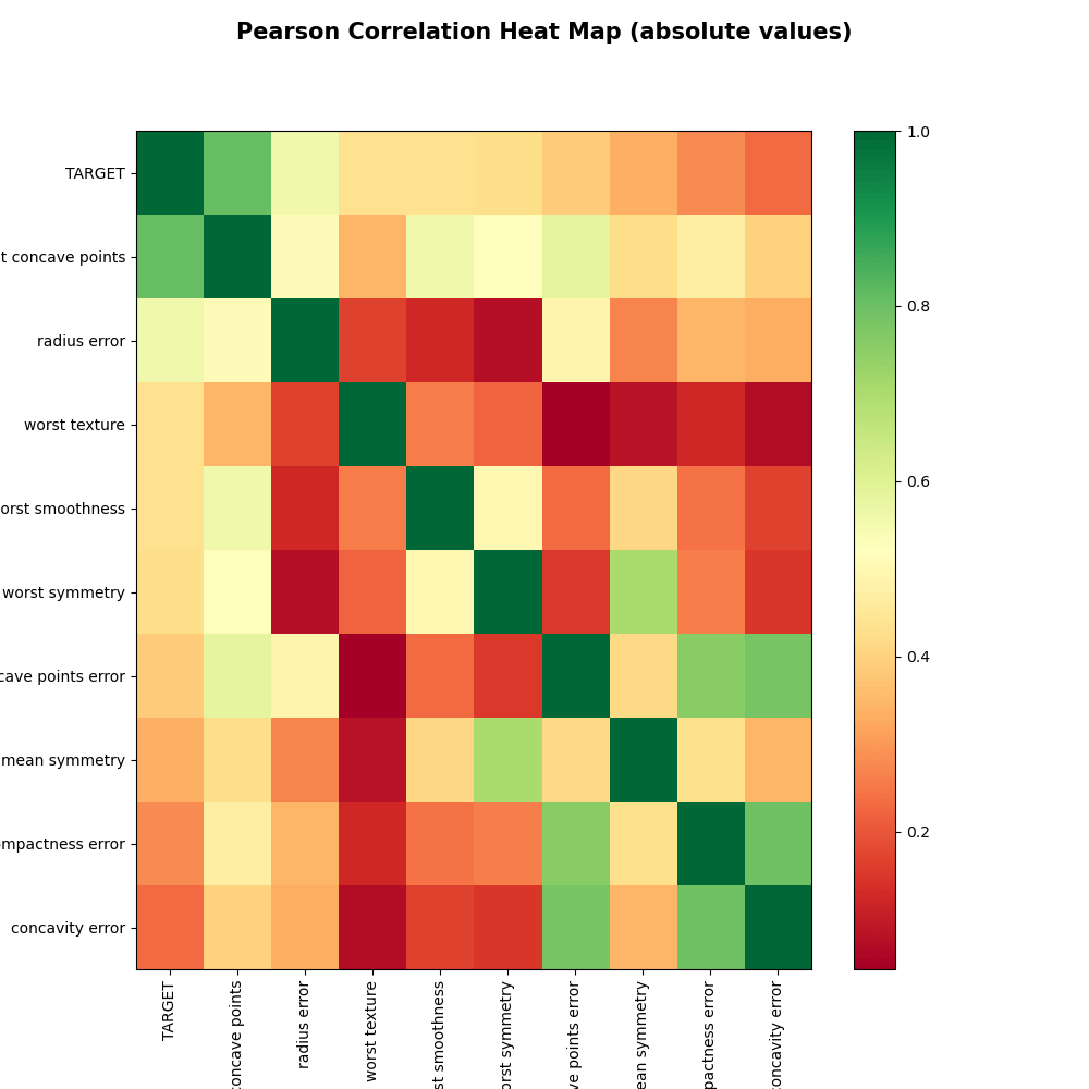
Let’s calculate the correlation matrix on the subset of features
X2 = X1[li_X2_cols]
print(“After the pair feature reduction, X2.shape:”, X2.shape)
yX2, yX_corr2, yX_abs_corr2 = correlation_matrix(y_train, X2)
Recalculate the correlation matrix to plot the TARGET values grouped by the order of correlation
s_X3_cols = yX_abs_corr2[‘TARGET’].sort_values(ascending=False)
li_X3_cols = s_X3_cols.index.tolist()
print(“Remaining features:”)
print(s_X3_cols)
print(“—“)
li_X3_cols.remove(‘TARGET’)
X3 = X2[li_X3_cols]
print(“After the pair feature reduction, X2.shape:”, X3.shape)
yX3, yX_corr3, yX_abs_corr3 = correlation_matrix(y_train, X3, is_plot=True)
X_train = X3
X_test = X_test_0[li_X3_cols]
After the pair feature reduction, X2.shape: (398, 9)
Function correlation_matrix: X.shape, y.shape, yX.shape: (398, 9) (398,) (398, 10)

Remaining features:
TARGET                  1.0000
worst concave points    0.8024
radius error            0.5574
worst texture           0.4347
worst smoothness        0.4324
worst symmetry          0.4255
concave points error    0.3902
mean symmetry           0.3361
compactness error       0.2823
concavity error         0.2322
Name: TARGET, dtype: float64
---
After the pair feature reduction, X2.shape: (398, 9)
Function correlation_matrix: X.shape, y.shape, yX.shape: (398, 9) (398,) (398, 10)
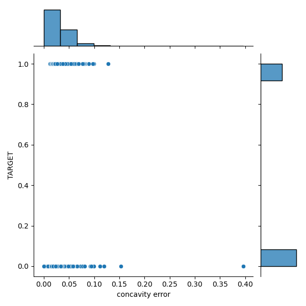
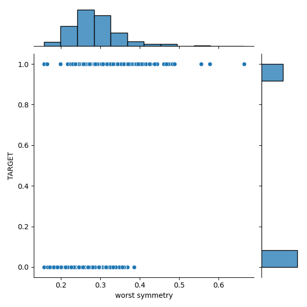
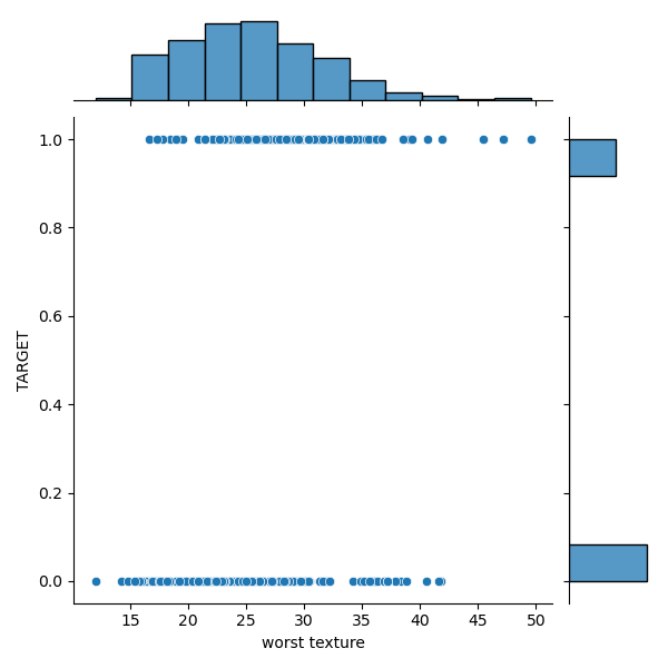
Let’s create the sns joint plot for the 9 remaining dominant features as follows:
sns.jointplot(yX3[‘concavity error’], yX3[‘TARGET’], kind=’scatter’, marginal_kws=dict(bins=12, rug=True))
plt.savefig(‘snsscatterconcavityerror.png’)
sns.jointplot(yX3[‘compactness error’], yX3[‘TARGET’], kind=’scatter’, marginal_kws=dict(bins=12, rug=True))
plt.savefig(‘snsscattercompactnesserror.png’)

sns.jointplot(yX3[‘mean symmetry’], yX3[‘TARGET’], kind=’scatter’, marginal_kws=dict(bins=12, rug=True))
plt.savefig(‘snsscattermeansymmetry.png’)

sns.jointplot(yX3[‘concave points error’], yX3[‘TARGET’], kind=’scatter’, marginal_kws=dict(bins=12, rug=True))
plt.savefig(‘snsscatterconcavepointserror.png’)

sns.jointplot(yX3[‘worst symmetry’], yX3[‘TARGET’], kind=’scatter’, marginal_kws=dict(bins=12, rug=True))
plt.savefig(‘snsscatterworstsymmetry.png’)
sns.jointplot(yX3[‘worst smoothness’], yX3[‘TARGET’], kind=’scatter’, marginal_kws=dict(bins=12, rug=True))
plt.savefig(‘snsscatterworstsmoothness.png’)

sns.jointplot(yX3[‘worst texture’], yX3[‘TARGET’], kind=’scatter’, marginal_kws=dict(bins=12, rug=True))
plt.savefig(‘snsscatterworsttexture.png’)
sns.jointplot(yX3[‘radius error’], yX3[‘TARGET’], kind=’scatter’, marginal_kws=dict(bins=12, rug=True))
plt.savefig(‘snsscatterradiuserror.png’)

sns.jointplot(yX3[‘worst concave points’], yX3[‘TARGET’], kind=’scatter’, marginal_kws=dict(bins=12, rug=True))
plt.savefig(‘snsscatterworstconcavepoints.png’)

We can see a significant overlap between the M and B distributions in the target-feature domain.
Let’s plot the joint scatter matrix of target and model features
color_map = {0: ‘#0392cf’, 1: ‘#7bc043’} # 0 (negative class): blue, 1 (positive class): green
colors = yX3[‘TARGET’].map(lambda x: color_map.get(x))
pd.plotting.scatter_matrix(yX3, alpha=0.5, color=colors, figsize=(16,18), diagonal=’hist’, hist_kwds={‘bins’:12})
plt.suptitle(‘Scatter matrix of target and model features’)
#plt.show()
plt.savefig(‘scattermatrixjointfeatures.png’)

Let’s print the train data and the class distribution of TARGET for both train and test sets
print(“X_train.shape, y_train.shape”, X_train.shape, y_train.shape)
val_cnts = y_train.value_counts()
print(“Class distribution of positive and negative samples in the train set:”)
print(val_cnts)
print(“Percentage of positive class samples: %s” % “%2f%%” % (100 * val_cnts[1] / len(y_train)))
print(“—“)
print(“X_test.shape, y_test.shape”, X_test.shape, y_test.shape)
val_cnts = y_test.value_counts()
print(“Class distribution of positive and negative samples in the test set:”)
print(val_cnts)
print(“Percentage of positive class samples: %s” % “%2f%%” % (100 * val_cnts[1] / len(y_test)))
X_train.shape, y_train.shape (398, 9) (398,)
Class distribution of positive and negative samples in the train set:
0    249
1    149
dtype: int64
Percentage of positive class samples: 37.437186%
---
X_test.shape, y_test.shape (171, 9) (171,)
Class distribution of positive and negative samples in the test set:
0    108
1     63
dtype: int64
Percentage of positive class samples: 36.842105%
Let’s define the HPO plotting function:
Plot 2d grid search heatmap
Parameters:
grid_search: instance of sklearn’s GridSearchCV
grid_params: dictionary of grid search parameters
x_param: name of x-axis parameter in grid_params
y_param: name of y-axis parameter in grid_params
is_verbose (optional): print results
Return:
grid_search.best_score_: best score found
grid_search.best_estimator_: best estimator found
def plot_2d_grid_search_heatmap(grid_search, grid_params, x_param, y_param, is_verbose=True):
grid_params_x = grid_params[x_param]
grid_params_y = grid_params[y_param]
df_results = pd.DataFrame(grid_search.cv_results_)
ar_scores = np.array(df_results.mean_test_score).reshape(len(grid_params_y), len(grid_params_x))
sns.heatmap(ar_scores, annot=True, fmt=’.3f’, xticklabels=grid_params_x, yticklabels=grid_params_y)
print()
plt.suptitle(‘Grid search heatmap’)
plt.xlabel(x_param)
plt.ylabel(y_param)
plt.savefig(“gridsearchheatmapgbm.png”)
if is_verbose:
print(“grid_search.best_score_:”)
print(grid_search.best_score_)
print()
print(“grid_search.best_estimator_:”)
print(grid_search.best_estimator_)
return grid_search.best_score_, grid_search.best_estimator_
Let’s run the LR classifier with GridSearchCV
grid_lr = {‘C’: [0.001, 0.01, 0.1, 1, 10, 100, 1000], ‘penalty’: [‘l1’, ‘l2’]}
clf_lr = LogisticRegression(class_weight=’balanced’, dual=False,
fit_intercept=True, intercept_scaling=1, max_iter=200,
n_jobs=1, random_state=0, tol=0.0001, verbose=0, warm_start=False)
gs_lr = GridSearchCV(clf_lr, grid_lr, return_train_score=True)
gs_lr.fit(X_train, y_train)
best_score_lr, clf_lr = plot_2d_grid_search_heatmap(gs_lr, grid_lr, ‘C’, ‘penalty’)
print(“intercept_:”)
print(clf_lr.intercept_ )
print()
print(“coef_:”)
print(clf_lr.coef_)
grid_search.best_score_:
0.9548417721518987

grid_search.best_estimator_:
LogisticRegression(C=1000, class_weight='balanced', max_iter=200, n_jobs=1,
                   random_state=0)
intercept_:
[-20.60103]

coef_:
[[ 78.14404612  15.64423206   0.25956452 -10.02229477  14.54515794
  -13.02308961 -13.84545081 -47.97567754 -12.68950602]]

Let’s run the GB classifier with GridSearchCV
grid_gb = {‘min_samples_leaf’: [2, 4, 8, 16], ‘learning_rate’: [0.001, 0.01, 0.1]}
clf_gbm = GradientBoostingClassifier(criterion=’friedman_mse’,
init=None, loss=’deviance’, max_features=’sqrt’, max_leaf_nodes=None,
max_depth=3, min_impurity_decrease=0.0,
min_samples_split=2, min_weight_fraction_leaf=0.0, n_estimators=800,
random_state=0, subsample=1.0, verbose=0, warm_start=False)
gs_gb = GridSearchCV(clf_gbm, grid_gb, verbose=0, return_train_score=True)
gs_gb.fit(X_train, y_train)
best_score_gb, clf_gb = plot_2d_grid_search_heatmap(gs_gb, grid_gb, ‘min_samples_leaf’, ‘learning_rate’)
grid_search.best_score_:
0.9447468354430381

grid_search.best_estimator_:
GradientBoostingClassifier(learning_rate=0.01, max_features='sqrt',
                           min_samples_leaf=2, n_estimators=800,
                           random_state=0)

Let’s create the std train data frame
dfimp = pd.DataFrame(np.std(X_train, 0), columns=[‘std’])
and calculate the importance factors to rank them from high to low values of importance
Logistic regression:
dfimp[‘coef’] = clf_lr.coef_.T
dfimp[‘lr_sign_imp’] = (np.std(X_train, 0).ravel() * clf_lr.coef_).T
dfimp[‘lr_imp’] = np.abs(dfimp[‘lr_sign_imp’])
GBM:
dfimp[‘gb_imp’] = pd.Series(clf_gb.feature_importances_, X_train.columns)
Add a column for the correlation with target
dfimp[‘target_corr’] = s_X3_cols.drop(‘TARGET’)
and perform ranking
dfimp[‘lr_rank’] = dfimp[‘lr_imp’].rank(ascending=False)
dfimp[‘gb_rank’] = dfimp[‘gb_imp’].rank(ascending=False)
dfimp[‘target_corr_rank’] = dfimp[‘target_corr’].rank(ascending=False)
dfsort = dfimp.sort_values(‘target_corr_rank’, ascending=True)
print(dfsort.iloc[:20,:].to_string())
                         std     coef  lr_sign_imp  lr_imp  gb_imp  target_corr  lr_rank  gb_rank  target_corr_rank
worst concave points  0.0656  78.1440       5.1267  5.1267  0.4893       0.8024      1.0      1.0               1.0
radius error          0.2936  15.6442       4.5931  4.5931  0.2137       0.5574      2.0      2.0               2.0
worst texture         6.1397   0.2596       1.5937  1.5937  0.0878       0.4347      3.0      3.0               3.0
worst smoothness      0.0230 -10.0223      -0.2301  0.2301  0.0400       0.4324      8.0      6.0               4.0
worst symmetry        0.0634  14.5452       0.9216  0.9216  0.0286       0.4255      4.0      7.0               5.0
concave points error  0.0059 -13.0231      -0.0762  0.0762  0.0567       0.3902      9.0      5.0               6.0
mean symmetry         0.0280 -13.8455      -0.3880  0.3880  0.0092       0.3361      6.0      9.0               7.0
compactness error     0.0168 -47.9757      -0.8066  0.8066  0.0141       0.2823      5.0      8.0               8.0
concavity error       0.0285 -12.6895      -0.3622  0.3622  0.0605       0.2322      7.0      4.0               9.0
Let’s look at the test data
cols_top = dfsort.index[:7]
print(“[y_test, X_test]”)
yX_test = pd.concat([y_test.iloc[-10:], X_test[cols_top].iloc[-10:,:]], axis=1)
yX_test = yX_test.rename(columns={0: ‘TARGET’})
print(yX_test.to_string())
[y_test, X_test]
     TARGET  worst concave points  radius error  worst texture  worst smoothness  worst symmetry  concave points error  mean symmetry
334       0                0.0398        0.1840          28.46            0.1222          0.2554                0.0065         0.1539
440       0                0.1555        0.2574          26.87            0.1391          0.2540                0.0177         0.1489
441       1                0.1739        0.5100          35.46            0.1436          0.2500                0.0174         0.1467
137       0                0.0848        0.1759          22.02            0.1190          0.2676                0.0086         0.1734
230       1                0.2543        0.2959          24.89            0.1703          0.3109                0.0138         0.2131
7         1                0.1556        0.5835          28.14            0.1654          0.3196                0.0145         0.2196
408       1                0.1974        0.4537          25.41            0.1482          0.3060                0.0148         0.1992
523       0                0.1284        0.3191          25.63            0.1425          0.2849                0.0135         0.1714
361       0                0.0561        0.2621          29.20            0.1140          0.2637                0.0064         0.1815
553       0                0.0256        0.3013          25.05            0.1103          0.2435                0.0128         0.1692
Let’s created the integrated LR-GBM HPO performance classification report
li_clfs = [‘clf_lr’, ‘clf_gb’]
dfp = pd.DataFrame(index=[‘TARGET’], data=[y_test]).T
for s_clf in li_clfs:
print(“MODEL: ” + s_clf)
print(“————–“)
clf = eval(s_clf)
y_pred = clf.predict(X_test).astype(int)  # returns a class decision based on the value of the predicted probability
y_score = clf.predict_proba(X_test)  # returns the value of the predicted probability

s_class = "%s_class" % s_clf
s_proba = "%s_proba" % s_clf
s_rank = "%s_rank" % s_clf

dfp[s_class] = y_pred
dfp[s_proba] = y_score[:,1]
dfp[s_rank] = dfp[s_proba].rank(ascending=1).astype(int)

# Print confusion matrix & classification report
# from sklearn.metrics import confusion_matrix
# cm = confusion_matrix(y_test, y_pred)

# Pandas 'crosstab' displays a better formatted confusion matrix than the one in sklearn
cm = pd.crosstab(y_test, y_pred, rownames=['Reality'], colnames=['Predicted'], margins=True)
print(cm)

print()
print("Classification report:")
print(classification_report(y_test, y_pred))
if s_clf == 'clf_lr':
    y_score_lr = y_score.copy()
elif s_clf == 'clf_gb':
    y_score_gb = y_score.copy()
else:
    print('Error')
    break
MODEL: clf_lr
--------------
Predicted    0   1  All
Reality
0          101   7  108
1            4  59   63
All        105  66  171

Classification report:
              precision    recall  f1-score   support

           0       0.96      0.94      0.95       108
           1       0.89      0.94      0.91        63

    accuracy                           0.94       171
   macro avg       0.93      0.94      0.93       171
weighted avg       0.94      0.94      0.94       171

MODEL: clf_gb
--------------
Predicted    0   1  All
Reality
0          103   5  108
1            7  56   63
All        110  61  171
Classification report:
              precision    recall  f1-score   support

           0       0.94      0.95      0.94       108
           1       0.92      0.89      0.90        63

    accuracy                           0.93       171
   macro avg       0.93      0.92      0.92       171
weighted avg       0.93      0.93      0.93       171
print(dfp.tail(10).to_string())
     TARGET  clf_lr_class  clf_lr_proba  clf_lr_rank  clf_gb_class  clf_gb_proba  clf_gb_rank
334       0             0        0.0006           30             0        0.0079           58
440       0             0        0.3821          101             1        0.7771          113
441       1             1        0.9994          137             1        0.9928          147
137       0             0        0.0020           44             0        0.0032            6
230       1             1        0.9998          147             1        0.9350          119
7         1             1        0.9975          131             1        0.9949          157
408       1             1        0.9990          135             1        0.9924          144
523       0             0        0.4748          105             0        0.2996          103
361       0             0        0.0035           52             0        0.0045           29
553       0             0        0.0001           13             0        0.0041           21
Let’s summarize the statistics
RANK_BINS = 10
rank_cols = [‘i_bin’, ‘i_min_bin’, ‘i_max_bin’, ‘score_min’, ‘score_max’, ‘bin_cnt’, ‘pos_cnt’, ‘pos_rate’]
rank_cols2 = [‘i_bin’, ‘score_min’, ‘score_max’, ‘tnr’, ‘fpr’, ‘fnr’, ‘tpr’, ‘tn’, ‘fp’, ‘fn’, ‘tp’]
print(dfp.shape)
len_test = dfp.shape[0]
len_bin = int(len_test / RANK_BINS)
for s_clf in li_clfs:
i_min_bin = 0
i_max_bin = 0
dfr = pd.DataFrame(columns=rank_cols)
dfr2 = pd.DataFrame(columns=rank_cols2)
s_class = "%s_class" % s_clf
s_proba = "%s_proba" % s_clf
s_rank = "%s_rank" % s_clf

for i in range(RANK_BINS):
    if i == RANK_BINS - 1:
        i_max_bin = len_test
    else:
        i_max_bin += len_bin

    # Range used for *each* score bin
    df_rng = dfp[(dfp[s_rank] >= i_min_bin) & (dfp[s_rank] < i_max_bin)]

    score_min = np.min(df_rng[s_proba])
    score_max = np.max(df_rng[s_proba])
    bin_cnt = df_rng.shape[0]

    pos_cnt = len(df_rng[df_rng['TARGET'] == 1])
    pos_rate = pos_cnt / bin_cnt

    # Range used for *all* score bins up to i_max_bin
    df_rng_0 = dfp[dfp[s_rank] < i_max_bin]
    df_rng_1 = dfp[dfp[s_rank] >= i_max_bin]

    # Positive targets (positive customers)
    tp = len(df_rng_1[df_rng_1['TARGET'] == 1])
    fn = len(df_rng_0[df_rng_0['TARGET'] == 1])
    pos = tp + fn
    tpr = tp / pos
    fnr = 1 - tpr

    # Negative targets
    tn = len(df_rng_0[df_rng_0['TARGET'] == 0])
    fp = len(df_rng_1[df_rng_1['TARGET'] == 0])
    neg = tn + fp
    fpr = fp / neg
    tnr = 1 - fpr

    # Build the dataframe for the summary stats per bin
    row = [i, i_min_bin, i_max_bin, score_min, score_max, bin_cnt, pos_cnt, pos_rate]
    dfr.loc[i] = row

    # Build the dataframe for the ROC stats per bin
    row2 = [i, score_min, score_max, tnr, fpr, fnr, tpr, tn, fp, fn, tp]
    dfr2.loc[i] = row2

    # Prep for next iteration
    i_min_bin = i_max_bin

if s_clf == 'clf_lr':
    dfr_lr = dfr.copy()
    dfr2_lr = dfr2.copy()
elif s_clf == 'clf_gb':
    dfr_gb = dfr.copy()
    dfr2_gb = dfr2.copy()
else:
    print('Error')
    break
print(“——-“)
print(“Results of positive count stats per bin”)
print(“Logistic Regression stats:”)
print(dfr_lr.to_string())
print()
print(“GBM stats:”)
print(dfr_gb.to_string())
print()
print(“—“)
print(“Overall stats in the test set:”)
pos_cnt = len(dfp[dfp[‘TARGET’] == 1])
pos_rate = pos_cnt / len_test
print(“pos_cnt”, pos_cnt)
print(“total rows”, len_test)
print(“pos_rate”, pos_rate)
(171, 7)
-------
Results of positive count stats per bin
Logistic Regression stats:
   i_bin  i_min_bin  i_max_bin   score_min  score_max  bin_cnt  pos_cnt  pos_rate
0    0.0        0.0       17.0  1.4302e-06     0.0002     16.0      0.0    0.0000
1    1.0       17.0       34.0  1.9229e-04     0.0007     17.0      0.0    0.0000
2    2.0       34.0       51.0  7.1944e-04     0.0033     17.0      0.0    0.0000
3    3.0       51.0       68.0  3.5092e-03     0.0103     17.0      0.0    0.0000
4    4.0       68.0       85.0  1.2065e-02     0.0481     17.0      1.0    0.0588
5    5.0       85.0      102.0  4.8669e-02     0.3821     17.0      3.0    0.1765
6    6.0      102.0      119.0  3.9533e-01     0.9029     17.0      6.0    0.3529
7    7.0      119.0      136.0  9.4799e-01     0.9990     17.0     17.0    1.0000
8    8.0      136.0      153.0  9.9925e-01     1.0000     17.0     17.0    1.0000
9    9.0      153.0      171.0  9.9999e-01     1.0000     18.0     18.0    1.0000

GBM stats:
   i_bin  i_min_bin  i_max_bin  score_min  score_max  bin_cnt  pos_cnt  pos_rate
0    0.0        0.0       17.0     0.0023     0.0040     16.0      0.0    0.0000
1    1.0       17.0       34.0     0.0040     0.0047     17.0      0.0    0.0000
2    2.0       34.0       51.0     0.0047     0.0058     17.0      0.0    0.0000
3    3.0       51.0       68.0     0.0059     0.0101     17.0      0.0    0.0000
4    4.0       68.0       85.0     0.0109     0.0341     17.0      2.0    0.1176
5    5.0       85.0      102.0     0.0362     0.2315     17.0      4.0    0.2353
6    6.0      102.0      119.0     0.2659     0.9298     17.0      5.0    0.2941
7    7.0      119.0      136.0     0.9350     0.9880     17.0     16.0    0.9412
8    8.0      136.0      153.0     0.9895     0.9945     17.0     17.0    1.0000
9    9.0      153.0      171.0     0.9946     0.9964     18.0     18.0    1.0000

---
Overall stats in the test set:
pos_cnt 63
total rows 171
pos_rate 0.3684210526315789
Let’s compare the percentiles for LR and GBM
s_titles = [‘Logistic Regression’, ‘GBM’]
plt.figure(figsize=(12, 4))
for i, s_clf in enumerate(li_clfs):
s_title = s_titles[i]
if s_clf == 'clf_lr':
    dfr = dfr_lr
    dfr2 = dfr2_lr
elif s_clf == 'clf_gb':
    dfr = dfr_gb
    dfr2 = dfr2_gb
else:
    print('Error')
    break

plt.subplot(1, 2, i+1)
plt.bar(dfr['i_bin'], dfr['pos_rate'])
plt.title('Percentiles for ' + s_title)

# Format charts
plt.grid()
plt.xlabel('Score bin (from low to high scoring bins)')
plt.ylabel('Ratio of positive classes per bin')
plt.legend(loc="lower right")

plt.xlim([0, RANK_BINS])
plt.ylim([0.0, 1])
#plt.show()
plt.savefig(“percentileslrgbm.png”)

It is clear that LR has the highest score and POS.
Let’s check the ROC curves
print(“Results of ROC stats per bin”)
print(“Logistic Regression stats:”)
print(dfr2_lr.to_string())
print()
print(“GBM stats:”)
print(dfr2_gb.to_string())
Results of ROC stats per bin
Logistic Regression stats:
   i_bin   score_min  score_max     tnr     fpr     fnr     tpr     tn    fp    fn    tp
0    0.0  1.4302e-06     0.0002  0.1481  0.8519  0.0000  1.0000   16.0  92.0   0.0  63.0
1    1.0  1.9229e-04     0.0007  0.3056  0.6944  0.0000  1.0000   33.0  75.0   0.0  63.0
2    2.0  7.1944e-04     0.0033  0.4630  0.5370  0.0000  1.0000   50.0  58.0   0.0  63.0
3    3.0  3.5092e-03     0.0103  0.6204  0.3796  0.0000  1.0000   67.0  41.0   0.0  63.0
4    4.0  1.2065e-02     0.0481  0.7685  0.2315  0.0159  0.9841   83.0  25.0   1.0  62.0
5    5.0  4.8669e-02     0.3821  0.8981  0.1019  0.0635  0.9365   97.0  11.0   4.0  59.0
6    6.0  3.9533e-01     0.9029  1.0000  0.0000  0.1587  0.8413  108.0   0.0  10.0  53.0
7    7.0  9.4799e-01     0.9990  1.0000  0.0000  0.4286  0.5714  108.0   0.0  27.0  36.0
8    8.0  9.9925e-01     1.0000  1.0000  0.0000  0.6984  0.3016  108.0   0.0  44.0  19.0
9    9.0  9.9999e-01     1.0000  1.0000  0.0000  0.9841  0.0159  108.0   0.0  62.0   1.0
GBM stats:
   i_bin  score_min  score_max     tnr     fpr     fnr     tpr     tn    fp    fn    tp
0    0.0     0.0023     0.0040  0.1481  0.8519  0.0000  1.0000   16.0  92.0   0.0  63.0
1    1.0     0.0040     0.0047  0.3056  0.6944  0.0000  1.0000   33.0  75.0   0.0  63.0
2    2.0     0.0047     0.0058  0.4630  0.5370  0.0000  1.0000   50.0  58.0   0.0  63.0
3    3.0     0.0059     0.0101  0.6204  0.3796  0.0000  1.0000   67.0  41.0   0.0  63.0
4    4.0     0.0109     0.0341  0.7593  0.2407  0.0317  0.9683   82.0  26.0   2.0  61.0
5    5.0     0.0362     0.2315  0.8796  0.1204  0.0952  0.9048   95.0  13.0   6.0  57.0
6    6.0     0.2659     0.9298  0.9907  0.0093  0.1746  0.8254  107.0   1.0  11.0  52.0
7    7.0     0.9350     0.9880  1.0000  0.0000  0.4286  0.5714  108.0   0.0  27.0  36.0
8    8.0     0.9895     0.9945  1.0000  0.0000  0.6984  0.3016  108.0   0.0  44.0  19.0
9    9.0     0.9946     0.9964  1.0000  0.0000  0.9841  0.0159  108.0   0.0  62.0   1.0
Let’s define and call the plot function
def plot_roc_and_precision_recall(y_true, y_score):
# Get ROC curve FPR and TPR from true labels vs score values
fpr, tpr, _ = roc_curve(y_true, y_score)
# Calculate ROC Area Under the Curve (AUC) from FPR and TPR data points
roc_auc = auc(fpr, tpr)
# Calculate precision and recall from true labels vs score values
precision, recall, _ = precision_recall_curve(y_true, y_score)
plt.figure(figsize=(8, 3))
plt.subplot(1,2,1)
lw = 2
plt.plot(fpr, tpr, color=’darkorange’, lw=lw, label=’ROC curve (AUC = %0.4f)’ % roc_auc)
plt.plot([0, 1], [0, 1], color=’navy’, lw=lw, linestyle=’–‘)
plt.xlim([0.0, 1.0])
plt.ylim([0.0, 1.05])
plt.xlabel(‘False Positive Rate’)
plt.ylabel(‘True Positive Rate’)
plt.title(‘ROC Curve’)
plt.legend(loc=”lower right”)
plt.grid(True)
plt.subplot(1,2,2)
plt.step(recall, precision, color=’orange’, where=’post’)
# plt.fill_between(recall, precision, step=’post’, alpha=0.5, color=’orange’)
plt.xlabel(‘Recall’)
plt.ylabel(‘Precision’)
plt.ylim([0.0, 1.05])
plt.xlim([0.0, 1.0])
plt.title(‘Precision Recall Curve’)
plt.grid(True)
left = 0.125 # the left side of the subplots of the figure
right = 0.9 # the right side of the subplots of the figure
bottom = 0.1 # the bottom part of the subplots of the figure
top = 0.9 # the top part of the subplots of the figure
wspace = 0.5 # the amount of width reserved for blank space between subplots
hspace = 0.2 # the amount of height reserved for white space between subplots
plt.subplots_adjust(left, bottom, right, top, wspace, hspace)
plt.show()
for s_clf in li_clfs:
print(“MODEL: ” + s_clf)
print(“————–“)
clf = eval(s_clf)
y_pred = clf.predict(X_test).astype(int)
y_score = clf.predict_proba(X_test)

plot_roc_and_precision_recall(y_test, y_score[:,1])  # provide the column for the scores belonging only to the positive class
print()
MODEL: clf_lr
--------------

MODEL: clf_gb
--------------
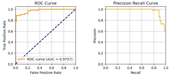
We can see that AUC(LR)>AUC(GBM).
Summary
- Train/test data splitting ratio 70:30%
- Feature engineering yields 9 dominant features
worst concave points 0.8024
radius error 0.5574
worst texture 0.4347
worst smoothness 0.4324
worst symmetry 0.4255
concave points error 0.3902
mean symmetry 0.3361
compactness error 0.2823
concavity error 0.2322
- LR Classification report:
- precision recall f1-score support
- 0 0.96 0.94 0.95 108
- 1 0.89 0.94 0.91 63
- accuracy 0.94 171
- GB Classification report:
- precision recall f1-score support
- 0 0.94 0.95 0.94 108
- 1 0.92 0.89 0.90 63
- accuracy 0.93 171
- Percentiles for LR vs GBM: LR has the highest score.
- AUC(LR)=0.987 > AUC(GBM)=0.975
- Results are consistent with the previous ML R&D study.
Read More
Colab Research Example using scikit-learn: Breast cancer prediction
A Comparative Analysis of Breast Cancer ML/AI Binary Classifications
Supervised ML/AI Breast Cancer Diagnostics (BCD) – The Power of HealthTech
How to find the importance of the features for a logistic regression model?


Make a one-time donation
Make a monthly donation
Make a yearly donation
Choose an amount
Or enter a custom amount
Your contribution is appreciated.
Your contribution is appreciated.
Your contribution is appreciated.

Leave a comment