Based on the Portfolio Optimization Algorithm (POA) discussed earlier and the related portfolio management, let’s run the Bear vs. Bull QC test of the portfolio P=[MSFT, AAPL, NDAQ] in terms of the Risk/Return Ratio (RRR).

Content:

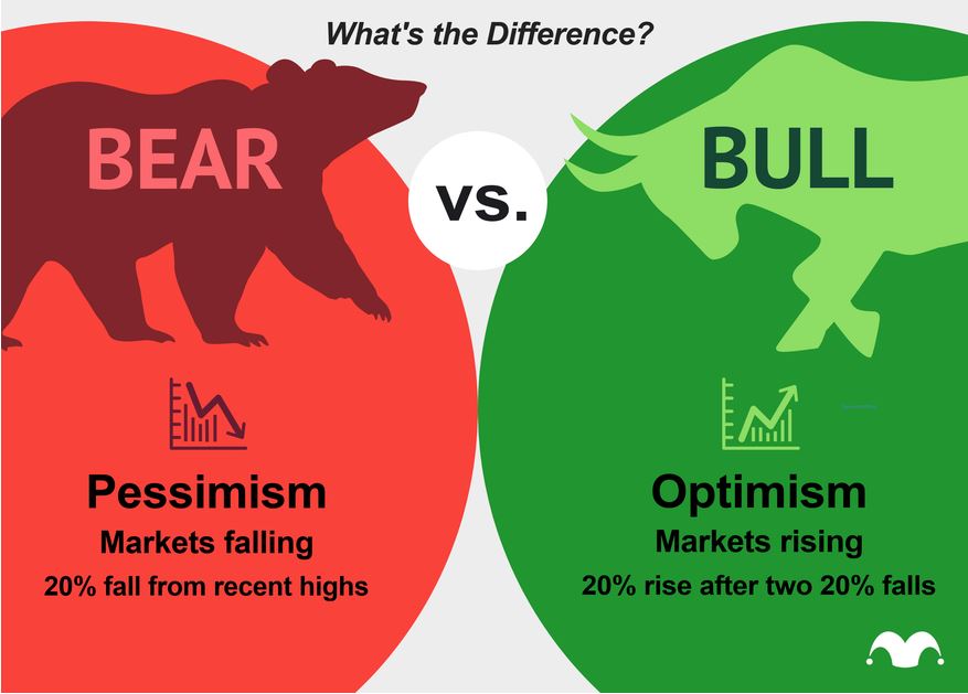
Stock prices are rising in a bull market and declining in a bear market. The stock market under bullish conditions is consistently gaining value, even with some brief market corrections. The stock market under bearish conditions is losing value or holding steady at depressed prices.

Low interest rates typically accompany bull markets, while high interest rates are associated with bear markets. Low interest rates make it more affordable for businesses to borrow money and grow, while high interest rates tend to slow companies’ expansions.

The Motley Fool Bear vs. Bull — **Source: The Motley Fool**

MSFT

The bears believe Microsoft’s business is still exposed to macroeconomic headwinds.
Wall Street remains overwhelmingly bullish on Microsoft. Analysts expect its revenue and adjusted earnings per share (EPS) to rise 19% and 16%, respectively, in fiscal 2022.
In fiscal 2023, they expect its revenue to increase 14% as its adjusted EPS grows another 16%.

AAPL

Bull case: Innovation spanning decades.
While Apple has done an excellent job creating sought-after consumer electronics like the iPod, iPad, AirPods, Apple Watch, etc., it’s still largely dependent on the iPhone.

In its most recent quarter, the iPhone comprised 52% of the company’s overall sales. That’s not even including all the attachments that go along with it. The risk is that if Apple doesn’t continue its iPhone success, revenue growth could stall or even reverse.

NDAQ

All three of the major U.S. stock indexes are now entrenched in a bear market.
While there’s no denying that bear markets can test the resolve of both tenured and new investors, history also shows that they’re the ideal opportunity to go hunting for bargains. No matter how bad things may appear for the leading indexes, a bull market rally eventually recoups all that was lost.

Barchart Opinion

Price Information

Company

Microsoft Corp

Apple Inc

Nasdaq Inc

Change

+8.57

+3.37

+0.47

% Change

+3.80%

+2.44%

+0.82%

Weighted Alpha

-27.20

-9.20

-10.80

A positive weighted alpha shows that the security produced a return greater than the benchmark; a negative measure indicates the converse.

Today’s Opinion

100% Sell

72% Sell

24% Buy

Performance 1-Month

%Chg

-7.51% since 09/13/22

-8.48% since 09/13/22

-6.11% since 09/13/22

Ratios

Price/Earnings ttm

24.50

22.93

22.49

The market average P/E ratio currently ranges from 20-25, so a higher PE above that could be considered bad, while a lower PE ratio could be considered better. A higher P/E ratio means you are paying more to purchase a share of the company’s earnings.

Comparison of MSFT (black), AAPL (blue), and NDAQ (orange) charts — **MSFT (black), AAPL (blue), and NDAQ (orange)** **charts**

Portfolio Allocation

Let’s set the working directory YOURPATH and import the key libraries

import os
os.chdir(‘C:/Users/adrou/OneDrive/Documents/PORTFOLIOJAYA’) # Set working directory
os. getcwd()
import numpy as np
import pandas as pd
import matplotlib.pyplot as plt
%matplotlib inline
import pandas_datareader.data as web
import datetime

Let’s define the time interval

start = datetime.datetime(2020,1,1)
end = datetime.datetime(2022,10,10)

and the 3 stock datasets

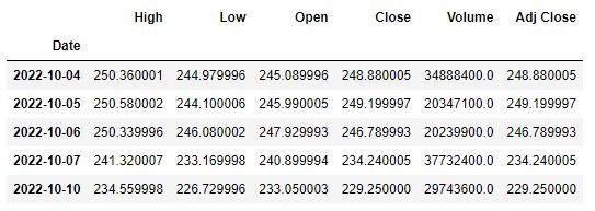
data1 = web.DataReader(‘MSFT’,’yahoo’,start,end)
data2 = web.DataReader(‘AAPL’,’yahoo’,start,end)
data3 = web.DataReader(‘NDAQ’,’yahoo’,start,end)

data1.tail()

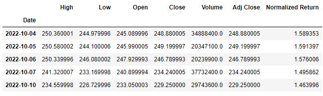
Let’s estimate normalized returns
for s_df in (data1,data2,data3):
s_df[‘Normalized Return’] = s_df[‘Adj Close’]/s_df.iloc[0][‘Adj Close’]

data1.tail()

Input MSFT stock data table with normalized returns

Allocations are as follows:
for s_df, allocation in zip((data1,data2,data3),[0.5,0.3,0.2]):
s_df[‘Allocation’] = s_df[‘Normalized Return’]*allocation

data1.tail()

Input MSFT stock data table with normalized returns and allocations

Let’s set

investment = 100000

and get the position value based on allocations

for s_df in (data1,data2,data3):
s_df[‘Position value’] = s_df[‘Allocation’] * investment

data1.tail()

Input MSFT stock data table with normalized returns and allocations + position values

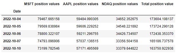
Now let’s look at the position values for all the stocks
position_values = pd.concat([data1[‘Position value’],
data2[‘Position value’],data3[‘Position value’]],axis=1)

position_values.columns = [‘MSFT position values’,’AAPL position values’,
‘NDAQ position values’]
position_values.tail()

The total position can now be calculated by summing the values of all stocks position values
position_values[‘Total position value’] = position_values.sum(axis=1)
position_values.tail()

position_values[‘Total position value’].plot(figsize=(10,8))
plt.title(‘Total portfolio value’)

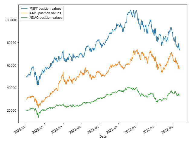
position_values.drop(‘Total position value’,axis=1).plot(figsize=(10,8))

Portfolio statistics:
position_values[‘Daily return’] = position_values[‘Total position value’].pct_change(1)
position_values.tail()

The mean daily return is given by

position_values[‘Daily return’].mean()

0.0009057958832049809

The Sharpe ratio is
sharpe_r = position_values[‘Daily return’].mean()/position_values[‘Daily return’].std()
sharpe_r

0.04543968353367672

and the annual Sharpe ratio is

annual_sharpe_r = sharpe_r * (252**0.5)
annual_sharpe_r

0.7213326137015117

Recall that A Sharpe ratio of less than one is considered unacceptable or bad. The risk your portfolio encounters isn’t being offset well enough by its return. The higher the Sharpe ratio, the better.

Portfolio Optimization

Let’s apply the revised portfolio management algorithm to our stocks. Firstly, the return will be plotted against volatility based on the Sharpe ratio. Secondly, the Python SciPy module will be used to create the return-volatility plot using the SLSQP optimization scheme.

Let’s continue the story by combining Adj Close columns of our 3 datasets

df1=data1[‘Adj Close’]
df2=data2[‘Adj Close’]
df3=data3[‘Adj Close’]
df = pd.concat([df1,df2,df3],axis=1)
df.columns = [‘MSFT’,’AAPL’,’NDAQ’]

df.tail()

Let’s check statistics.

Mean daily return:

Using the percent change function, the mean daily return of the stocks is
df.pct_change(1).mean()

MSFT    0.000780
AAPL    0.001190
NDAQ    0.000929
dtype: float64

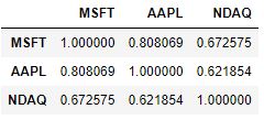
The mean daily return yields the degree of correlation between the stocks

df.pct_change(1).corr()

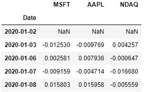
The percentage change method also gives the arithmetic return

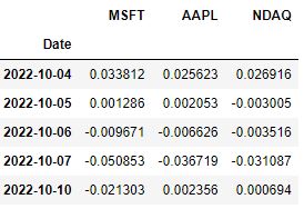
or in log scale

log_returns = np.log(df/df.shift(1))
log_returns.head()

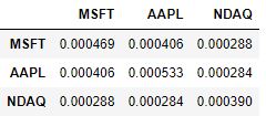
Hence, the covariance matrix is

log_returns.cov()

Optimization via Randomization – Allocation of random weights to the stocks. The weights are randomly allocated to the stocks and made sure that they all add up to 1. To make sure they add up to 1, the weights are rebalanced by dividing it by the sum of weights:

print(‘The stocks are: ‘,df.columns)
np.random.seed(200)
weights = np.array(np.random.random(3)) #random weights
weights = weights/np.sum(weights)
print(‘Random weights: ‘,weights)

The stocks are:  Index(['MSFT', 'AAPL', 'NDAQ'], dtype='object')
Random weights:  [0.53580931 0.12809422 0.33609646]

The annual expected return is

expected_return = np.sum((log_returns.mean()* weights) * 252)
expected_return

0.16570984130750205

The annual expected volatility is

expected_vol = np.sqrt(np.dot(weights.T,np.dot(log_returns.cov()*252,weights)))
expected_vol

0.3059477823851022

Hence, the Sharpe ratio is

sharpe_r = expected_return/expected_vol
sharpe_r

0.541627855628383

Let’s run the random optimization algorithm

np.random.seed(200)

Initalization of variables

portfolio_number = 7000
weights_total = np.zeros((portfolio_number,len(df.columns)))
returns = np.zeros(portfolio_number)
volatility = np.zeros(portfolio_number)
sharpe = np.zeros(portfolio_number)

for i in range(portfolio_number):

# Random weights
weights = np.array(np.random.random(3))
weights = weights/np.sum(weights)
# Append weight
weights_total[i,:] = weights

# Expected return
returns[i] = np.sum((log_returns.mean()* weights) * 252)

# Expected volume
volatility[i] = np.sqrt(np.dot(weights.T,np.dot(log_returns.cov()*252,weights)))

# Sharpe ratio
sharpe[i] = returns[i]/volatility[i]

Let’s calculate the max Sharpe ratio

max_sharpe = sharpe.max()
max_sharpe

0.6818731773912419

max_sharpe_index = sharpe.argmax()
max_sharpe_index

max_sharpe_weights = weights_total[343,:]
max_sharpe_weights

array([6.71707148e-01, 2.83931652e-04, 3.28008920e-01])

Let’s calculate the corresponding max expected return and volatility

max_sharpe_return = returns[max_sharpe_index]
max_sharpe_return

0.21046030001983235

max_sharpe_vol = volatility[max_sharpe_index]
max_sharpe_vol

0.3086502109160916

Let’s plot the Return-Volatility map as the scatter plot

plt.figure(figsize=(12,8))
plt.scatter(volatility,returns,c=sharpe)
plt.colorbar(label=’Sharpe Ratio’)
plt.xlabel(‘Volatility’)
plt.ylabel(‘Return’)

plt.scatter(max_sharpe_vol,max_sharpe_return,c=’red’,s=50)

Random optimization return-volatility vs Sharpe ratio scatter plot

Let’s apply the SLSQP minimization algorithm from scipy.optimize (with constraints, bounds, and the initial guess as input parameters) to verify this result

def stats(weights):
weights = np.array(weights)
expected_return = np.sum((log_returns.mean()* weights) * 252)
expected_vol = np.sqrt(np.dot(weights.T,np.dot(log_returns.cov()*252,weights)))
sharpe_r = expected_return/expected_vol
return np.array([expected_return,expected_vol,sharpe_r])

from scipy.optimize import minimize

def sr_negate(weights):
neg_sr = stats(weights)[2] * -1
return neg_sr
def weight_check(weights):
weights_sum = np.sum(weights)
return weights_sum – 1

constraints = ({‘type’:’eq’,’fun’:weight_check})
bounds = ((0,1),(0,1),(0,1))
initial_guess = [0.3,0.3,0.4]

results = minimize(sr_negate,initial_guess,method=’SLSQP’,bounds=bounds,constraints=constraints)
results

fun: -0.6819487289981644
     jac: array([ 1.87360495e-01, -1.54420733e-04,  1.82241201e-04])
 message: 'Optimization terminated successfully'
    nfev: 20
     nit: 5
    njev: 5
  status: 0
 success: True
       x: array([1.48788148e-16, 5.41313619e-01, 4.58686381e-01])

wt = results.x
wt
stats(wt)

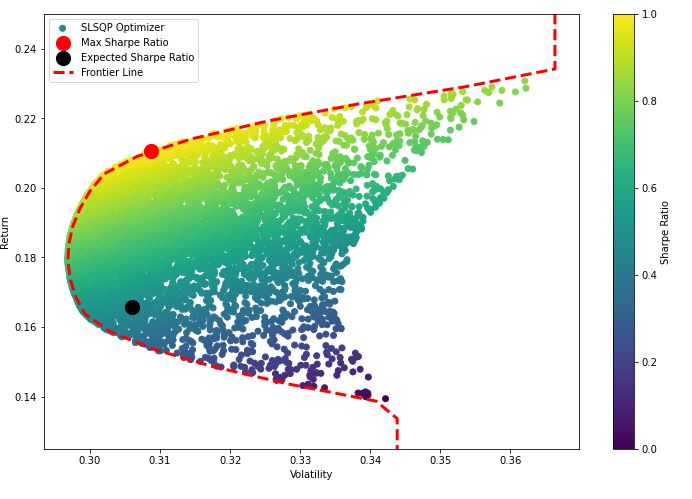
Let’s plot the Return-Volatility map with the volatility frontier envelope

frontier_return = np.linspace(-0.6,0.4,200)
def min_vol(weights):
vol = stats(weights)[1]
return vol
frontier_volatility = []

for exp_return in frontier_return:
constraints = ({‘type’:’eq’,’fun’:weight_check},
{‘type’:’eq’,’fun’:lambda x: stats(x)[0]-exp_return})
result = minimize(min_vol,initial_guess,method=’SLSQP’,bounds=bounds,constraints=constraints)
frontier_volatility.append(result[‘fun’])

plt.figure(figsize=(12,8))
plt.scatter(volatility,returns,c=sharpe)
plt.scatter(max_sharpe_vol,max_sharpe_return,c=’red’,s=200)
plt.scatter(expected_vol,expected_return,c=’black’,s=200)
plt.colorbar(label=’Sharpe Ratio’)
plt.xlabel(‘Volatility’)
plt.ylabel(‘Return’)

plt.plot(frontier_volatility,frontier_return,’r–‘,linewidth=3)
plt.legend([‘SLSQP Optimizer’, ‘Max Sharpe Ratio’,’Expected Sharpe Ratio’,’Frontier Line’])
plt.ylim([0.125, 0.25])

Summary

Portfolio & Timing

start = datetime.datetime(2020,1,1)
end = datetime.datetime(2022,10,10)

and the 3 stock datasets imported from Yahoo Finance

web.DataReader(‘MSFT’,’yahoo’,start,end)
web.DataReader(‘AAPL’,’yahoo’,start,end)
web.DataReader(‘NDAQ’,’yahoo’,start,end)

Volatility (Max Sharpe Ratio) ~ Volatility (Expected Sharpe Ratio) ~ 0.31
Return (Max Sharpe Ratio) ~ 0.21 > Return (Expected Sharpe Ratio) ~ 0.17
Expected Sharpe Ratio ~ 0.54 < 1.0
Volatility: var(MSFT) ~4.69e-4 > var(AAPL) ~4.1e-4 > var(NDAQ)~2.9e-4
Similarity index corr(MSFT,AAPL)~0.81 > corr(MSFT,NAQ)~0.67 ~ corr(AAPL,NAQ) ~0.62
the mean daily return of the stocks is (AAPL>MSFT>NDAQ)

MSFT 0.000780

AAPL 0.001190

NDAQ 0.000929

Conclusions

A Sharpe ratio of less than one is considered unacceptable or bad. The risk the portfolio P encounters isn’t being offset well enough by its return.
The expected return of the portfolio P is lower than the return associated with Max Sharpe Ratio.
Poor diversification: three stocks follow more or less the similar trend, as confirmed by the relatively high correlation coefficient above 0.5 and a similar value of variance
Stocks have a similar degree of volatility, as shown by their variance
The outcome is consistent with the stock-to-sell barchart.com opinion (see above).