An AWS Comparison of ML/AI Diabetes-2 Classification Algorithms

Featured Photo by Myriam Zilles on Unsplash

In the last decade, the impact of Type-2 Diabetes (T2D) has increased to a great extent especially in developing countries. Therefore, early diagnosis and classification of T2D has become an active area of healthtech. Numerous data-driven techniques are available to control T2D. This work presents a comparative use-case study of several exploratory data analysis (EDA) and ML/AI algorithms which process T2D data effectively. The existing Python workflows are analyzed in a comprehensive manner to identify their pros and cons. Their performance assessment is carried out to determine the best approach.

Contents:

1. Background
2. State-of-the-Art
3. Workflow
4. Data
5. The AWS Approach
6. Conclusions
7. References
8. Explore More

Background

• T2D is a common condition that causes the level of sugar (glucose) in the blood to become too high. T2D is responsible for very considerable morbidity, mortality. Furthermore, it is a substantial financial drain health systems and societies. 
• Early diagnosis is important to reduce the incidence and mortality rate of diabetes.
• Screening tools have been developed to identify individuals at high risk of developing T2D.
• Most screening tests for T2D in use today were developed using electronically collected data from Electronic Health Record (EHR).
• Traditional screening approaches are based on standard regression techniques.
• It is important to investigate whether using advanced data-based approaches can yield superior results to the currently employed methods.

• The increasing volume of EHR opened the opportunity to develop more accurate AI-driven prediction models that can be continuously updated using available ML algorithms. 

State-of-the-Art

Over the last years, various ML/AI techniques (DNN, SVM, KNN, DT, GBT, GBM, RF, LR, etc.) have been used to predict T2D and its complications. However, researchers and developers still face two main challenges when building T2D predictive models:

• There is considerable heterogeneity in previous studies regarding algorithms used, making it challenging to identify the optimal one.
• There is a lack of transparency about the features used in the optimized models, which reduces their interpretability.
• This systematic analysis aimed at providing answers to the above challenges.
• The study followed the earlier review primarily, enriched with the most recent case studies (cf. References and Explore More).

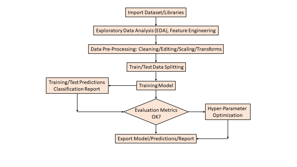
Workflow

Data

Conventionally, T2D ML/AI studies use the Kaggle PIMA Indian Diabetes (PID) dataset taken from the National Institute of Diabetes and Kidney Diseases center, see UC Irvine Machine Learning Repository. The objective of the dataset is to diagnostically predict whether or not a patient has diabetes, based on certain diagnostic measurements included in the dataset. Several constraints were placed on the selection of these instances from a larger database. In particular, all patients here are females at least 21 years old of Pima Indian heritage.

The AWS Approach

Let’s Import libraries
import numpy as np # linear algebra
import pandas as pd # data processing, CSV file I/O (e.g. pd.read_csv)
import seaborn as sns # for data visualization
import matplotlib.pyplot as plt # to plot charts
from collections import Counter
import os

from sklearn.preprocessing import QuantileTransformer
from sklearn.metrics import confusion_matrix, accuracy_score, precision_score
from sklearn.ensemble import RandomForestClassifier, AdaBoostClassifier, GradientBoostingClassifier, VotingClassifier
from sklearn.linear_model import LogisticRegression
from sklearn.neighbors import KNeighborsClassifier
from sklearn.tree import DecisionTreeClassifier
from sklearn.svm import SVC
from sklearn.model_selection import GridSearchCV, cross_val_score, StratifiedKFold, learning_curve, train_test_split

Let’s import the input dataset

df = pd.read_csv(“diabetes.csv”)

and get familier with dataset structure
df.info()

0   Pregnancies               768 non-null    int64  
 1   Glucose                   768 non-null    int64  
 2   BloodPressure             768 non-null    int64  
 3   SkinThickness             768 non-null    int64  
 4   Insulin                   768 non-null    int64  
 5   BMI                       768 non-null    float64
 6   DiabetesPedigreeFunction  768 non-null    float64
 7   Age                       768 non-null    int64  
 8   Outcome                   768 non-null    int64  
dtypes: float64(2), int64(7)

Let’s look at top 5 rows
df.head()

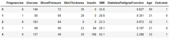
Our target variable is Outcome.

Let’s explore missing values if any
df.isnull().sum()

Pregnancies                 0
Glucose                     0
BloodPressure               0
SkinThickness               0
Insulin                     0
BMI                         0
DiabetesPedigreeFunction    0
Age                         0
Outcome                     0
dtype: int64

There are no missing values.

Let’s review the dataset descriptive statistics
df.describe()

and look at the correlation matrix

plt.figure(figsize=(13,10))
sns.heatmap(df.corr(),annot=True, fmt = “.2f”, cmap = “coolwarm”)

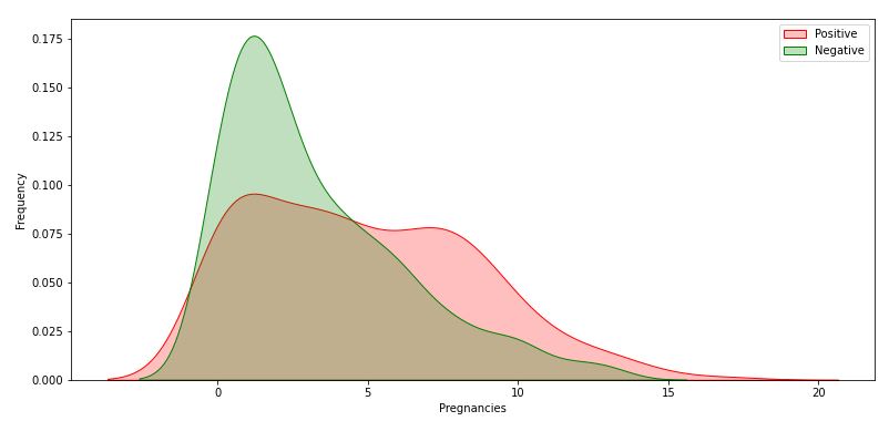
Let’s explore Pregnancies vs Outcome
plt.figure(figsize=(13,6))
g = sns.kdeplot(df[“Pregnancies”][df[“Outcome”] == 1],
color=”Red”, shade = True)
g = sns.kdeplot(df[“Pregnancies”][df[“Outcome”] == 0],
ax =g, color=”Green”, shade= True)
g.set_xlabel(“Pregnancies”)
g.set_ylabel(“Frequency”)
g.legend([“Positive”,”Negative”])

Let’s explore Glucose vs Outcome
plt.figure(figsize=(10,6))
sns.violinplot(data=df, x=”Outcome”, y=”Glucose”,
split=True, inner=”quart”, linewidth=1)

Let’s explore Glucose vs Outcome empirical distributions

plt.figure(figsize=(13,6))
g = sns.kdeplot(df[“Glucose”][df[“Outcome”] == 1], color=”Red”, shade = True)
g = sns.kdeplot(df[“Glucose”][df[“Outcome”] == 0], ax =g, color=”Green”, shade= True)
g.set_xlabel(“Glucose”)
g.set_ylabel(“Frequency”)
g.legend([“Positive”,”Negative”])

Let’s combine Glucose vs BMI vs Age

plt.figure(figsize=(20,10))
sns.scatterplot(data=df, x=”Glucose”, y=”BMI”, hue=”Age”, size=”Age”)

Let’s detect outliers

def detect_outliers(df,n,features):
outlier_indices = []
“””
Detect outliers from given list of features. It returns a list of the indices
according to the observations containing more than n outliers according
to the Tukey method
“””
# iterate over features(columns)
for col in features:
Q1 = np.percentile(df[col], 25)
Q3 = np.percentile(df[col],75)
IQR = Q3 – Q1

    # outlier step
    outlier_step = 1.5 * IQR

    # Determine a list of indices of outliers for feature col
    outlier_list_col = df[(df[col] < Q1 - outlier_step) | (df[col] > Q3 + outlier_step )].index

    # append the found outlier indices for col to the list of outlier indices 
    outlier_indices.extend(outlier_list_col)

# select observations containing more than 2 outliers
outlier_indices = Counter(outlier_indices)
multiple_outliers = list( k for k, v in outlier_indices.items() if v > n )

return multiple_outliers 

Let’s group outliers to drop using the above function

outliers_to_drop = detect_outliers(df, 2 ,[“Pregnancies”, ‘Glucose’, ‘BloodPressure’, ‘BMI’, ‘DiabetesPedigreeFunction’, ‘SkinThickness’, ‘Insulin’, ‘Age’])

We are ready to drop those outliers

df.drop(df.loc[outliers_to_drop].index, inplace=True)

Let’s apply the QuantileTransformer to change the probability distribution of numeric variables to improve the performance of predictive models

q = QuantileTransformer()
X = q.fit_transform(df)
transformedDF = q.transform(X)
transformedDF = pd.DataFrame(X)
transformedDF.columns =[‘Pregnancies’, ‘Glucose’, ‘BloodPressure’, ‘SkinThickness’, ‘Insulin’, ‘BMI’, ‘DiabetesPedigreeFunction’, ‘Age’, ‘Outcome’]

Let’s look at top 5 rows of the transformed dataset
transformedDF.head()

Let’s separate features and labels

features = df.drop([“Outcome”], axis=1)
labels = df[“Outcome”]

Let’s perform training/test data split with test_size=0.30

x_train, x_test, y_train, y_test = train_test_split(features, labels, test_size=0.30, random_state=7)

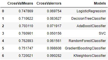
Let’s evaluate ML models using the function

def evaluate_model(models):
“””
Takes a list of models and returns chart of cross validation scores using mean accuracy
“””

# Cross validate model with Kfold stratified cross val
kfold = StratifiedKFold(n_splits = 10)

result = []
for model in models :
    result.append(cross_val_score(estimator = model, X = x_train, y = y_train, scoring = "accuracy", cv = kfold, n_jobs=4))

cv_means = []
cv_std = []
for cv_result in result:
    cv_means.append(cv_result.mean())
    cv_std.append(cv_result.std())

result_df = pd.DataFrame({
    "CrossValMeans":cv_means,
    "CrossValerrors": cv_std,
    "Models":[
        "LogisticRegression",
        "DecisionTreeClassifier",
        "AdaBoostClassifier",
        "SVC",
        "RandomForestClassifier",
        "GradientBoostingClassifier",
        "KNeighborsClassifier"
    ]
})

# Generate chart
bar = sns.barplot(x = "CrossValMeans", y = "Models", data = result_df, orient = "h")
bar.set_xlabel("Mean Accuracy")
bar.set_title("Cross validation scores")
return result_df

Let’s perform modeling to compare different algorithms
random_state = 30
models = [
LogisticRegression(random_state = random_state, solver=’liblinear’),
DecisionTreeClassifier(random_state = random_state),
AdaBoostClassifier(DecisionTreeClassifier(random_state = random_state), random_state = random_state, learning_rate = 0.2),
SVC(random_state = random_state),
RandomForestClassifier(random_state = random_state),
GradientBoostingClassifier(random_state = random_state),
KNeighborsClassifier(),
]
evaluate_model(models)

Let’s implement hyper-parameter optimization (HPO) via GridSearchCV and print out the classification report

from sklearn.model_selection import GridSearchCV
from sklearn.metrics import classification_report
def analyze_grid_result(grid_result):
”’
Analysis of GridCV result and predicting with test dataset
Show classification report at last
”’
# Best parameters and accuracy
print(“Tuned hyperparameters: (best parameters) “, grid_result.best_params_)
print(“Accuracy :”, grid_result.best_score_)

means = grid_result.cv_results_["mean_test_score"]
stds = grid_result.cv_results_["std_test_score"]
for mean, std, params in zip(means, stds, grid_result.cv_results_["params"]):
    print("%0.3f (+/-%0.03f) for %r" % (mean, std * 2, params))
print()
print("Detailed classification report:")
y_true, y_pred = y_test, grid_result.predict(x_test)
print(classification_report(y_true, y_pred))
print()

Let’s define models and parameters for LogisticRegression
model = LogisticRegression(solver=’liblinear’)
solvers = [‘newton-cg’, ‘liblinear’]
penalty = [‘l2’]
c_values = [100, 10, 1.0, 0.1, 0.01]

Let’s consider GridSearchCV HPO
grid = dict(solver = solvers, penalty = penalty, C = c_values)
cv = StratifiedKFold(n_splits = 50, random_state = 1, shuffle = True)
grid_search = GridSearchCV(estimator = model, param_grid = grid, cv = cv, scoring = ‘accuracy’, error_score = 0)
logi_result = grid_search.fit(x_train, y_train)

Let’s print out the Logistic Regression HPO Result
analyze_grid_result(logi_result)

Tuned hyperparameters: (best parameters)  {'C': 10, 'penalty': 'l2', 'solver': 'liblinear'}
Accuracy : 0.7883636363636363
0.788 (+/-0.260) for {'C': 100, 'penalty': 'l2', 'solver': 'newton-cg'}
0.788 (+/-0.260) for {'C': 100, 'penalty': 'l2', 'solver': 'liblinear'}
0.788 (+/-0.260) for {'C': 10, 'penalty': 'l2', 'solver': 'newton-cg'}
0.788 (+/-0.250) for {'C': 10, 'penalty': 'l2', 'solver': 'liblinear'}
0.785 (+/-0.253) for {'C': 1.0, 'penalty': 'l2', 'solver': 'newton-cg'}
0.743 (+/-0.267) for {'C': 1.0, 'penalty': 'l2', 'solver': 'liblinear'}
0.773 (+/-0.238) for {'C': 0.1, 'penalty': 'l2', 'solver': 'newton-cg'}
0.705 (+/-0.281) for {'C': 0.1, 'penalty': 'l2', 'solver': 'liblinear'}
0.773 (+/-0.232) for {'C': 0.01, 'penalty': 'l2', 'solver': 'newton-cg'}
0.696 (+/-0.264) for {'C': 0.01, 'penalty': 'l2', 'solver': 'liblinear'}

Detailed classification report:
              precision    recall  f1-score   support

           0       0.78      0.84      0.81       147
           1       0.68      0.58      0.62        83

    accuracy                           0.75       230
   macro avg       0.73      0.71      0.72       230
weighted avg       0.74      0.75      0.74       230

Let’s look at the GridSearchCV

model = SVC()

tuned_parameters = [
{“kernel”: [“rbf”], “gamma”: [1e-3, 1e-4], “C”: [1, 10, 100, 1000]},
{“kernel”: [“linear”], “C”: [1, 10, 100, 1000]},
]
cv = StratifiedKFold(n_splits = 2, random_state = 1, shuffle = True)
grid_search = GridSearchCV(estimator = model, param_grid = tuned_parameters, cv = cv, scoring = ‘accuracy’, error_score = 0)
scv_result = grid_search.fit(x_train, y_train)

analyze_grid_result(scv_result)

Tuned hyperparameters: (best parameters)  {'C': 10, 'kernel': 'linear'}
Accuracy : 0.7775797976410084
0.712 (+/-0.061) for {'C': 1, 'gamma': 0.001, 'kernel': 'rbf'}
0.735 (+/-0.053) for {'C': 1, 'gamma': 0.0001, 'kernel': 'rbf'}
0.677 (+/-0.035) for {'C': 10, 'gamma': 0.001, 'kernel': 'rbf'}
0.716 (+/-0.016) for {'C': 10, 'gamma': 0.0001, 'kernel': 'rbf'}
0.658 (+/-0.020) for {'C': 100, 'gamma': 0.001, 'kernel': 'rbf'}
0.707 (+/-0.042) for {'C': 100, 'gamma': 0.0001, 'kernel': 'rbf'}
0.656 (+/-0.001) for {'C': 1000, 'gamma': 0.001, 'kernel': 'rbf'}
0.667 (+/-0.046) for {'C': 1000, 'gamma': 0.0001, 'kernel': 'rbf'}
0.770 (+/-0.025) for {'C': 1, 'kernel': 'linear'}
0.778 (+/-0.010) for {'C': 10, 'kernel': 'linear'}
0.778 (+/-0.005) for {'C': 100, 'kernel': 'linear'}
0.759 (+/-0.033) for {'C': 1000, 'kernel': 'linear'}

Detailed classification report:
              precision    recall  f1-score   support

           0       0.78      0.84      0.81       147
           1       0.67      0.57      0.61        83

    accuracy                           0.74       230
   macro avg       0.72      0.70      0.71       230
weighted avg       0.74      0.74      0.74       230

Let’s look at the RandomForestClassifier HPO

model = RandomForestClassifier(random_state=42)

tuned_parameters = {
‘n_estimators’: [200, 500],
‘max_features’: [‘auto’, ‘sqrt’, ‘log2’],
‘max_depth’ : [4,5,6,7,8],
‘criterion’ :[‘gini’, ‘entropy’]
}
cv = StratifiedKFold(n_splits = 2, random_state = 1, shuffle = True)
grid_search = GridSearchCV(estimator = model, param_grid = tuned_parameters, cv = cv, scoring = ‘accuracy’, error_score = 0)
grid_result = grid_search.fit(x_train, y_train)

analyze_grid_result(grid_result)

Tuned hyperparameters: (best parameters)  {'criterion': 'entropy', 'max_depth': 5, 'max_features': 'log2', 'n_estimators': 200}
Accuracy : 0.7663648051875454
0.759 (+/-0.025) for {'criterion': 'gini', 'max_depth': 4, 'max_features': 'auto', 'n_estimators': 200}
0.761 (+/-0.029) for {'criterion': 'gini', 'max_depth': 4, 'max_features': 'auto', 'n_estimators': 500}
0.759 (+/-0.025) for {'criterion': 'gini', 'max_depth': 4, 'max_features': 'sqrt', 'n_estimators': 200}
0.761 (+/-0.029) for {'criterion': 'gini', 'max_depth': 4, 'max_features': 'sqrt', 'n_estimators': 500}
0.751 (+/-0.018) for {'criterion': 'gini', 'max_depth': 4, 'max_features': 'log2', 'n_estimators': 200}
0.757 (+/-0.022) for {'criterion': 'gini', 'max_depth': 4, 'max_features': 'log2', 'n_estimators': 500}
0.751 (+/-0.025) for {'criterion': 'gini', 'max_depth': 5, 'max_features': 'auto', 'n_estimators': 200}
0.759 (+/-0.025) for {'criterion': 'gini', 'max_depth': 5, 'max_features': 'auto', 'n_estimators': 500}
0.751 (+/-0.025) for {'criterion': 'gini', 'max_depth': 5, 'max_features': 'sqrt', 'n_estimators': 200}
0.759 (+/-0.025) for {'criterion': 'gini', 'max_depth': 5, 'max_features': 'sqrt', 'n_estimators': 500}
0.751 (+/-0.025) for {'criterion': 'gini', 'max_depth': 5, 'max_features': 'log2', 'n_estimators': 200}
0.753 (+/-0.014) for {'criterion': 'gini', 'max_depth': 5, 'max_features': 'log2', 'n_estimators': 500}
0.763 (+/-0.033) for {'criterion': 'gini', 'max_depth': 6, 'max_features': 'auto', 'n_estimators': 200}
0.757 (+/-0.029) for {'criterion': 'gini', 'max_depth': 6, 'max_features': 'auto', 'n_estimators': 500}
0.763 (+/-0.033) for {'criterion': 'gini', 'max_depth': 6, 'max_features': 'sqrt', 'n_estimators': 200}
0.757 (+/-0.029) for {'criterion': 'gini', 'max_depth': 6, 'max_features': 'sqrt', 'n_estimators': 500}
0.759 (+/-0.025) for {'criterion': 'gini', 'max_depth': 6, 'max_features': 'log2', 'n_estimators': 200}
0.753 (+/-0.029) for {'criterion': 'gini', 'max_depth': 6, 'max_features': 'log2', 'n_estimators': 500}
0.755 (+/-0.033) for {'criterion': 'gini', 'max_depth': 7, 'max_features': 'auto', 'n_estimators': 200}
0.751 (+/-0.025) for {'criterion': 'gini', 'max_depth': 7, 'max_features': 'auto', 'n_estimators': 500}
0.755 (+/-0.033) for {'criterion': 'gini', 'max_depth': 7, 'max_features': 'sqrt', 'n_estimators': 200}
0.751 (+/-0.025) for {'criterion': 'gini', 'max_depth': 7, 'max_features': 'sqrt', 'n_estimators': 500}
0.748 (+/-0.018) for {'criterion': 'gini', 'max_depth': 7, 'max_features': 'log2', 'n_estimators': 200}
0.746 (+/-0.007) for {'criterion': 'gini', 'max_depth': 7, 'max_features': 'log2', 'n_estimators': 500}
0.751 (+/-0.033) for {'criterion': 'gini', 'max_depth': 8, 'max_features': 'auto', 'n_estimators': 200}
0.751 (+/-0.040) for {'criterion': 'gini', 'max_depth': 8, 'max_features': 'auto', 'n_estimators': 500}
0.751 (+/-0.033) for {'criterion': 'gini', 'max_depth': 8, 'max_features': 'sqrt', 'n_estimators': 200}
0.751 (+/-0.040) for {'criterion': 'gini', 'max_depth': 8, 'max_features': 'sqrt', 'n_estimators': 500}
0.750 (+/-0.021) for {'criterion': 'gini', 'max_depth': 8, 'max_features': 'log2', 'n_estimators': 200}
0.757 (+/-0.044) for {'criterion': 'gini', 'max_depth': 8, 'max_features': 'log2', 'n_estimators': 500}
0.763 (+/-0.040) for {'criterion': 'entropy', 'max_depth': 4, 'max_features': 'auto', 'n_estimators': 200}
0.759 (+/-0.040) for {'criterion': 'entropy', 'max_depth': 4, 'max_features': 'auto', 'n_estimators': 500}
0.763 (+/-0.040) for {'criterion': 'entropy', 'max_depth': 4, 'max_features': 'sqrt', 'n_estimators': 200}
0.759 (+/-0.040) for {'criterion': 'entropy', 'max_depth': 4, 'max_features': 'sqrt', 'n_estimators': 500}
0.757 (+/-0.029) for {'criterion': 'entropy', 'max_depth': 4, 'max_features': 'log2', 'n_estimators': 200}
0.763 (+/-0.010) for {'criterion': 'entropy', 'max_depth': 4, 'max_features': 'log2', 'n_estimators': 500}
0.757 (+/-0.022) for {'criterion': 'entropy', 'max_depth': 5, 'max_features': 'auto', 'n_estimators': 200}
0.757 (+/-0.036) for {'criterion': 'entropy', 'max_depth': 5, 'max_features': 'auto', 'n_estimators': 500}
0.757 (+/-0.022) for {'criterion': 'entropy', 'max_depth': 5, 'max_features': 'sqrt', 'n_estimators': 200}
0.757 (+/-0.036) for {'criterion': 'entropy', 'max_depth': 5, 'max_features': 'sqrt', 'n_estimators': 500}
0.766 (+/-0.010) for {'criterion': 'entropy', 'max_depth': 5, 'max_features': 'log2', 'n_estimators': 200}
0.764 (+/-0.014) for {'criterion': 'entropy', 'max_depth': 5, 'max_features': 'log2', 'n_estimators': 500}
0.765 (+/-0.022) for {'criterion': 'entropy', 'max_depth': 6, 'max_features': 'auto', 'n_estimators': 200}
0.763 (+/-0.033) for {'criterion': 'entropy', 'max_depth': 6, 'max_features': 'auto', 'n_estimators': 500}
0.765 (+/-0.022) for {'criterion': 'entropy', 'max_depth': 6, 'max_features': 'sqrt', 'n_estimators': 200}
0.763 (+/-0.033) for {'criterion': 'entropy', 'max_depth': 6, 'max_features': 'sqrt', 'n_estimators': 500}
0.764 (+/-0.007) for {'criterion': 'entropy', 'max_depth': 6, 'max_features': 'log2', 'n_estimators': 200}
0.759 (+/-0.025) for {'criterion': 'entropy', 'max_depth': 6, 'max_features': 'log2', 'n_estimators': 500}
0.761 (+/-0.014) for {'criterion': 'entropy', 'max_depth': 7, 'max_features': 'auto', 'n_estimators': 200}
0.757 (+/-0.022) for {'criterion': 'entropy', 'max_depth': 7, 'max_features': 'auto', 'n_estimators': 500}
0.761 (+/-0.014) for {'criterion': 'entropy', 'max_depth': 7, 'max_features': 'sqrt', 'n_estimators': 200}
0.757 (+/-0.022) for {'criterion': 'entropy', 'max_depth': 7, 'max_features': 'sqrt', 'n_estimators': 500}
0.757 (+/-0.029) for {'criterion': 'entropy', 'max_depth': 7, 'max_features': 'log2', 'n_estimators': 200}
0.753 (+/-0.014) for {'criterion': 'entropy', 'max_depth': 7, 'max_features': 'log2', 'n_estimators': 500}
0.755 (+/-0.010) for {'criterion': 'entropy', 'max_depth': 8, 'max_features': 'auto', 'n_estimators': 200}
0.755 (+/-0.025) for {'criterion': 'entropy', 'max_depth': 8, 'max_features': 'auto', 'n_estimators': 500}
0.755 (+/-0.010) for {'criterion': 'entropy', 'max_depth': 8, 'max_features': 'sqrt', 'n_estimators': 200}
0.755 (+/-0.025) for {'criterion': 'entropy', 'max_depth': 8, 'max_features': 'sqrt', 'n_estimators': 500}
0.748 (+/-0.040) for {'criterion': 'entropy', 'max_depth': 8, 'max_features': 'log2', 'n_estimators': 200}
0.763 (+/-0.033) for {'criterion': 'entropy', 'max_depth': 8, 'max_features': 'log2', 'n_estimators': 500}

Detailed classification report:
              precision    recall  f1-score   support

           0       0.78      0.83      0.80       147
           1       0.66      0.58      0.62        83

    accuracy                           0.74       230
   macro avg       0.72      0.70      0.71       230
weighted avg       0.73      0.74      0.74       230

Let’s test logi_result predictions
y_pred = logi_result.predict(x_test)
print(classification_report(y_test, y_pred))

precision    recall  f1-score   support

           0       0.78      0.84      0.81       147
           1       0.68      0.58      0.62        83

    accuracy                           0.75       230
   macro avg       0.73      0.71      0.72       230
weighted avg       0.74      0.75      0.74       230

Let’s add our predictions to the test dataset

x_test[‘pred’] = y_pred
print(x_test)

 Pregnancies  Glucose  BloodPressure  SkinThickness  Insulin   BMI  
236            7    181.0           84.0             21    192.0  35.9   
715            7    187.0           50.0             33    392.0  33.9   
766            1    126.0           60.0             23     30.5  30.1   
499            6    154.0           74.0             32    193.0  29.3   
61             8    133.0           72.0             23     30.5  32.9   
..           ...      ...            ...            ...      ...   ...   
189            5    139.0           80.0             35    160.0  31.6   
351            4    137.0           84.0             23     30.5  31.2   
120            0    162.0           76.0             56    100.0  53.2   
108            3     83.0           58.0             31     18.0  34.3   
637            2     94.0           76.0             18     66.0  31.6   

     DiabetesPedigreeFunction  Age  pred  
236                     0.586   51     1  
715                     0.826   34     1  
766                     0.349   47     0  
499                     0.839   39     1  
61                      0.270   39     1  
..                        ...  ...   ...  
189                     0.361   25     0  
351                     0.252   30     0  
120                     0.759   25     1  
108                     0.336   25     0  
637                     0.649   23     0  

[230 rows x 9 columns]

Let’s plot histograms

plt.hist(y_test)

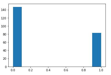
plt.hist(y_pred)

Conclusions

• Input dataset: the Kaggle PIMA Indian Diabetes (PID)
• Data Pre-Processing: drop outliers and apply QuantileTransformer
• Correlation matrix feature ranking: 1 – Glucose, 2 – BMI, 3 – Age.
• 0.7 < Cross-Validation Mean Errors (Models) < 0.8
• Binary Classification Models: LR, KNN, GB, RF, DT, AdaBoost, and SVC.
• SVC HPO via GridSearchCV: Accuracy : 0.77

precision recall f1-score support

0 0.78 0.84 0.81 147

1 0.67 0.57 0.61 83

• RandomForestClassifier HPO via GridSearchCV: Accuracy : 0.74

precision recall f1-score support

0 0.78 0.83 0.80 147

1 0.66 0.58 0.62 83

References

Machine learning and deep learning predictive models for type 2 diabetes: a systematic review

Early detection of type 2 diabetes mellitus using machine learning-based prediction models

Explore More

About

HealthTech ML/AI Q3 ’22 Round-Up

The Application of ML/AI in Diabetes

Diabetes Prediction using ML/AI in Python

HealthTech ML/AI Use-Cases