ML/AI Credit Risk Analytics

This project was inspired by the multi-classification proof-of-concept research in the area of credit risk analytics (CRA). CRA provides a guide for risk managers looking to efficiently build credit risk management models.  In recent studies, credit rating models have been constructed by relying on a number of financial ratios, including correlations between them.

The input dataset ratings.csv can be downloaded from the Github repository. The corresponding CRA code is also available.

Featured Photo by Jonathan Cooper on Unsplash.

Workflow:

• Import libraries and download input data
• Data Editing and Exploratory Data Analysis (EDA)
• Feature Engineering (FE) and importance scores
• Training/Testing multi-classification models
• ML validation and QC performance analysis
• Saving the best model and classification report

Contents:

1. Preparation Phase + EDA
2. Building Model + FE + QC
3. Performance
4. Summary

Preparation Phase + EDA

Let’s set the working directory YOURPATH

import os
os.chdir(‘YOURPATH’)
os. getcwd()

import the key libraries

import pandas as pd
import numpy as np

import scikitplot as skplt

import sklearn
from sklearn.datasets import load_digits, load_boston, load_breast_cancer
from sklearn.model_selection import train_test_split

from sklearn.ensemble import RandomForestClassifier, RandomForestRegressor, GradientBoostingClassifier, ExtraTreesClassifier
from sklearn.linear_model import LinearRegression, LogisticRegression
from sklearn.cluster import KMeans
from sklearn.decomposition import PCA

import itertools

import matplotlib.pyplot as plt

import sys
import warnings
warnings.filterwarnings(“ignore”)

print(“Scikit Plot Version : “, skplt.version)
print(“Scikit Learn Version : “, sklearn.version)
print(“Python Version : “, sys.version)

%matplotlib inline

Scikit Plot Version :  0.3.7
Scikit Learn Version :  1.0.2
Python Version :  3.9.12 (main, Apr  4 2022, 05:22:27)

import seaborn as sns

from sklearn.model_selection import train_test_split

from sklearn.neighbors import KNeighborsClassifier

from sklearn.linear_model import LogisticRegression

from sklearn.tree import DecisionTreeClassifier

from sklearn.ensemble import RandomForestClassifier

from sklearn.ensemble import GradientBoostingClassifier

from sklearn.svm import SVC

from sklearn.preprocessing import StandardScaler

from sklearn.neural_network import MLPClassifier

from sklearn.linear_model import LogisticRegression

from sklearn.metrics import confusion_matrix

from sklearn.metrics import classification_report

and download the input dataset

df = pd.read_csv(“ratings.csv”)
print(df.columns)

Index(['spid', 'rating', 'COMMEQTA', 'LLPLOANS', 'COSTTOINCOME', 'ROE',
       'LIQASSTA', 'SIZE'],
      dtype='object')

df.head()

df.shape

(5000, 8)

df.info()
<class 'pandas.core.frame.DataFrame'>
RangeIndex: 5000 entries, 0 to 4999
Data columns (total 8 columns):
 #   Column        Non-Null Count  Dtype  
---  ------        --------------  -----  
 0   spid          5000 non-null   int64  
 1   rating        5000 non-null   int64  
 2   COMMEQTA      5000 non-null   float64
 3   LLPLOANS      5000 non-null   float64
 4   COSTTOINCOME  5000 non-null   float64
 5   ROE           5000 non-null   float64
 6   LIQASSTA      5000 non-null   float64
 7   SIZE          5000 non-null   float64
dtypes: float64(6), int64(2)
memory usage: 312.6 KB

Let’s drop the column spid

df.drop([‘spid’], axis=1, inplace=True)

df.columns

Index(['rating', 'COMMEQTA', 'LLPLOANS', 'COSTTOINCOME', 'ROE', 'LIQASSTA',
       'SIZE'],
      dtype='object')
Let's create the sns pairplot

Let’s separate the feature and target columns

X = df.loc[:, df.columns != “rating”]
y = df.loc[:, df.columns == “rating”]

and split the data into training/testing subsets with test_size=0.2

X_train, X_test, y_train, y_test = train_test_split(X, y, test_size=0.2, random_state=42, stratify=y)

Building Model + FE + QC

Let’s look at KNeighborsClassifier

training_accuracy = []
test_accuracy = []

try n_neighbors from 1 to 10

neighbors_settings = range(1, 11)
for n_neighbors in neighbors_settings:

fit the classification model with the above parameters

knn = KNeighborsClassifier(n_neighbors=n_neighbors)
knn.fit(X_train, y_train)

check the training set accuracy
training_accuracy.append(knn.score(X_train, y_train))

and the test set accuracy
test_accuracy.append(knn.score(X_test, y_test))

plt.plot(neighbors_settings, training_accuracy, label=”training accuracy”)
plt.plot(neighbors_settings, test_accuracy, label=”test accuracy”)
plt.ylabel(“Accuracy”)
plt.xlabel(“n_neighbors”)
plt.legend()
plt.savefig(“knn_compare_model”)

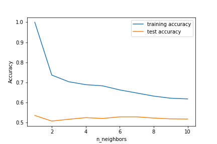
Let’s run the model with the optimal set n_neighbors=4

knn = KNeighborsClassifier(n_neighbors=4)
knn.fit(X_train, y_train)
print(“Accuracy of K-NN classifier on training set: {:.2f}”.format(knn.score(X_train, y_train)))
print(“Accuracy of K-NN classifier on test set: {:.2f}”.format(knn.score(X_test, y_test)))

Accuracy of K-NN classifier on training set: 0.69
Accuracy of K-NN classifier on test set: 0.53

let’s look at the KNN learning curve

skplt.estimators.plot_learning_curve(knn, X, y,
cv=7, shuffle=True, scoring=”accuracy”,
n_jobs=-1, figsize=(6,4), title_fontsize=”large”, text_fontsize=”large”,
title=”KNeighborsClassifier() Learning Curve”);

Let’s compare it to LogisticRegression

logreg = LogisticRegression(random_state=42).fit(X_train, y_train)
print(“Training set score: {:.3f}”.format(logreg.score(X_train, y_train)))
print(“Test set score: {:.3f}”.format(logreg.score(X_test, y_test)))

Training set score: 0.462
Test set score: 0.463

Let’s check it against DecisionTreeClassifier

tree1 = DecisionTreeClassifier(random_state=42)
tree1.fit(X_train, y_train)
print(“Accuracy on training set: {:.3f}”.format(tree1.score(X_train, y_train)))
print(“Accuracy on test set: {:.3f}”.format(tree1.score(X_test, y_test)))

Accuracy on training set: 1.000
Accuracy on test set: 0.708

Let’s update the parameteres to avoid training set overfitting

tree2 = DecisionTreeClassifier(max_depth=10, random_state=1)
tree2.fit(X_train, y_train)
print(“Accuracy on training set: {:.3f}”.format(tree2.score(X_train, y_train)))
print(“Accuracy on test set: {:.3f}”.format(tree2.score(X_test, y_test)))

Accuracy on training set: 0.812
Accuracy on test set: 0.742

The corresponding learning curve looks as follows:

skplt.estimators.plot_learning_curve(tree2, X, y,
cv=7, shuffle=True, scoring=”accuracy”,
n_jobs=-1, figsize=(6,4), title_fontsize=”large”, text_fontsize=”large”,
title=”DecisionTreeClassifier() Learning Curve”);

This is the best result so far.

Let’s plot Feature importances

df_features = [x for i,x in enumerate(X.columns) if i!= len(X.columns) ]
print(“Feature importances:\n{}”.format(tree2.feature_importances_))

Feature importances:
[0.09359034 0.26028331 0.1721998  0.17193909 0.09117593 0.21081153]

def plot_feature_importances_credit(model):
plt.figure(figsize=(8,6))
n_features = len(X.columns)
plt.barh(range(n_features), model.feature_importances_, align=’center’)
plt.yticks(np.arange(n_features), df_features)
plt.xlabel(“Feature importance”)
plt.ylabel(“Feature”)
plt.ylim(-1, n_features)

plot_feature_importances_credit(tree2)
plt.savefig(‘feature_importance.png’)

We can see that LLPLOANS appears to be the most dominant feature.

Let’s look at RandomForestClassifier

rf = RandomForestClassifier(n_estimators=100, random_state=42)
rf.fit(X_train, y_train)
print(“Accuracy on training set: {:.3f}”.format(rf.score(X_train, y_train)))
print(“Accuracy on test set: {:.3f}”.format(rf.score(X_test, y_test)))

Accuracy on training set: 1.000
Accuracy on test set: 0.799

Let’s update the parameters

rf1 = RandomForestClassifier(max_depth=18, n_estimators=100, random_state=1)
rf1.fit(X_train, y_train)
print(“Accuracy on training set: {:.3f}”.format(rf1.score(X_train, y_train)))
print(“Accuracy on test set: {:.3f}”.format(rf1.score(X_test, y_test)))

Accuracy on training set: 0.978
Accuracy on test set: 0.800

It appears that RandomForestClassifier is more accurate than DecisionTreeClassifier.

Let’s plot feature importances

plot_feature_importances_credit(rf1)

Let’s run GradientBoostingClassifier

gb2 = GradientBoostingClassifier(learning_rate=0.2, random_state=1)
gb2.fit(X_train, y_train)
print(“Accuracy on training set: {:.3f}”.format(gb2.score(X_train, y_train)))
print(“Accuracy on test set: {:.3f}”.format(gb2.score(X_test, y_test)))

Accuracy on training set: 0.970
Accuracy on test set: 0.817

The feature importance chart is

plot_feature_importances_credit(gb2)

Let’s apply the SVC algorithm to the data scaled by StandardScaler

scaler = StandardScaler()
X_train_scaled = scaler.fit_transform(X_train)
X_test_scaled = scaler.fit_transform(X_test)
svc2 = SVC(C=500, random_state=42)
svc2.fit(X_train_scaled, y_train)
print(“Accuracy on training set: {:.2f}”.format(svc2.score(X_train_scaled, y_train)))
print(“Accuracy on test set: {:.2f}”.format(svc2.score(X_test_scaled, y_test)))

Accuracy on training set: 0.90
Accuracy on test set: 0.71

Let’s compare it to MLPClassifier

X_train_scaled = scaler.fit_transform(X_train)
X_test_scaled = scaler.fit_transform(X_test)
mlp3 = MLPClassifier(max_iter=5000, random_state=42)
mlp3.fit(X_train_scaled, y_train)
print(“Accuracy on training set: {:.3f}”.format(mlp3.score(X_train_scaled, y_train)))
print(“Accuracy on test set: {:.3f}”.format(mlp3.score(X_test_scaled, y_test)))

Accuracy on training set: 0.836
Accuracy on test set: 0.764

Let’s look at the NN weight coefficients

plt.figure(figsize=(20, 5))
plt.imshow(mlp3.coefs_[0], interpolation=”none”, cmap=’viridis’)
plt.yticks(range(len(X.columns)), df_features)
plt.xlabel(“Columns in weight matrix”)
plt.ylabel(“Input feature”)
plt.colorbar()

Finally, let’s try LogisticRegression

logreg100 = LogisticRegression(C=10, random_state=42).fit(X_train, y_train)
print(“Training set accuracy: {:.3f}”.format(logreg100.score(X_train, y_train)))
print(“Test set accuracy: {:.3f}”.format(logreg100.score(X_test, y_test)))

Training set accuracy: 0.488
Test set accuracy: 0.480

Let’s get the summary of tests accuracy

algorithms = [“k-Nearest Neighbors”, “Logistic Regression”, “Decision Trees”, “Random Forest”,
“Gradient Boosting”, “Support Vector Machine”, “Deep Learning”]

tests_accuracy = [knn.score(X_test, y_test), logreg100.score(X_test, y_test), tree2.score(X_test, y_test),
rf1.score(X_test, y_test), gb2.score(X_test, y_test), svc2.score(X_test_scaled, y_test),
mlp3.score(X_test_scaled, y_test)]

compare_algorithms = pd.DataFrame({ “Algorithms”: algorithms, “Tests Accuracy”: tests_accuracy })
compare_algorithms.sort_values(by = “Tests Accuracy”, ascending = False)

Let’s plot this table as the bar chart

import matplotlib.pyplot as plt
%matplotlib inline
plt.figure(figsize=(8,8))
sns.barplot(x = “Tests Accuracy”, y = “Algorithms”, data = compare_algorithms)
plt.show()

The Gradient Boosting (GB) algorithm gives us the sense of achieving the highest test accuracy of 81.7%.

Performance

Let’s check the GB model performance

model = gb2
model

GradientBoostingClassifier(learning_rate=0.2, random_state=1)

Let’s make test GB predictions

predictions = model.predict(X_test)

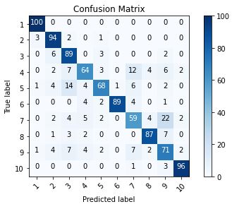
and compute the GB confusion matrix

cm = confusion_matrix(y_true=y_test, y_pred=predictions)

Let’s define the following plot function

def plot_confusion_matrix(cm, classes,
normalize=False,
title=’Confusion matrix’,
cmap=plt.cm.Blues):
“””
This function prints and plots the confusion matrix.
Normalization can be applied by setting normalize=True.
“””
plt.imshow(cm, interpolation=’nearest’, cmap=cmap)
plt.title(title)
plt.colorbar()
tick_marks = np.arange(len(classes))
plt.xticks(tick_marks, classes, rotation=45)
plt.yticks(tick_marks, classes)

if normalize:
    cm = cm.astype('float') / cm.sum(axis=1)[:, np.newaxis]
    print("Normalized confusion matrix")
else:
    print('Confusion matrix, without normalization')

print(cm)

thresh = cm.max() / 2.
for i, j in itertools.product(range(cm.shape[0]), range(cm.shape[1])):
    plt.text(j, i, cm[i, j],
        horizontalalignment="center",
        color="white" if cm[i, j] > thresh else "black")

plt.tight_layout()
plt.ylabel('True label')
plt.xlabel('Predicted label')

Let’s plot the GB confusion matrix with the labels

cm_plot_labels = [‘1′,’2′,’3′,’4′,’5′,’6′,’7′,’8′,’9′,’10’]
plot_confusion_matrix(cm=cm, classes=cm_plot_labels, title=’Confusion Matrix’)

Let’s print our predictions

print(“\033[1m The result is telling us that we have: “,(cm[0,0] + cm[1,1] + cm[2,2] + cm[3,3] + cm[4,4] +
cm[5,5] + cm[6,6] + cm[7,7] + cm[8,8] + cm[9,9] ),”correct predictions.”)
print(“\033[1m The result is telling us that we have: “, ( cm.sum() – (cm[0,0] + cm[1,1] + cm[2,2] +
cm[3,3] + cm[4,4] + cm[5,5] + cm[6,6] + cm[7,7] +
cm[8,8] + cm[9,9] )),”incorrect predictions.”)
print(“\033[1m We have a total predictions of: “,( cm.sum()) )

The result is telling us that we have:  817 correct predictions (81.7%).
The result is telling us that we have:  183 incorrect predictions (18.3%).
We have a total predictions of:  1000

Let’s print the multi-classification report

print(classification_report(y_test, predictions))

precision    recall  f1-score   support

           1       0.95      1.00      0.98       100
           2       0.83      0.94      0.88       100
           3       0.71      0.89      0.79       100
           4       0.77      0.64      0.70       100
           5       0.84      0.68      0.75       100
           6       0.99      0.89      0.94       100
           7       0.66      0.59      0.62       100
           8       0.90      0.87      0.88       100
           9       0.62      0.71      0.66       100
          10       0.94      0.96      0.95       100

    accuracy                           0.82      1000
   macro avg       0.82      0.82      0.82      1000
weighted avg       0.82      0.82      0.82      1000

Let’s plot the GB learning curve

skplt.estimators.plot_learning_curve(gb2, X, y,
cv=7, shuffle=True, scoring=”accuracy”,
n_jobs=-1, figsize=(6,4), title_fontsize=”large”, text_fontsize=”large”,
title=”GradientBoostingClassifier() Learning Curve”);

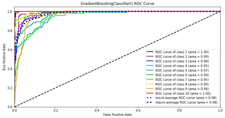
Let’s plot the GB ROC curve

Y_test_probs = gb2.predict_proba(X_test)

skplt.metrics.plot_roc_curve(y_test, Y_test_probs,
title=”GradientBoostingClassifier() ROC Curve”, figsize=(12,6));

skplt.metrics.plot_precision_recall_curve(y_test, Y_test_probs,
title=”GradientBoostingClassifier() Precision-Recall Curve”, figsize=(12,6));

Let’s look at the GB elbow plot

skplt.cluster.plot_elbow_curve(KMeans(random_state=1),
X_train,
cluster_ranges=range(2, 20),
figsize=(8,6));

Let’s perform the KMeans cluster analysis

kmeans = KMeans(n_clusters=10, random_state=1)
kmeans.fit(X_train, y_train)
cluster_labels = kmeans.predict(X_test)

skplt.metrics.plot_silhouette(X_test, cluster_labels,
figsize=(8,6));

Let’s look at the PCA components

pca = PCA(random_state=1)
pca.fit(X_train)

skplt.decomposition.plot_pca_component_variance(pca, figsize=(8,6));

Summary

• Machine Learning (ML) algorithms have been used to classify multiple outcomes in credit ratings datasets, including random forests (RF), KNeighbors (KNN), decision tree (DT), Gradient Boosting (GB), logistic regression (LR), artificial neural networks (ANN), and support vector machine (SVM). 
• The Gradient Boosting (GB) algorithm has given us the sense of achieving the highest test accuracy of 81.7%.
• The GB multi-classification report consists of 10 labels:

label precision recall f1-score support

1 0.95 1.00 0.98 100

2 0.83 0.94 0.88 100

3 0.71 0.89 0.79 100

4 0.77 0.64 0.70 100

5 0.84 0.68 0.75 100

6 0.99 0.89 0.94 100

7 0.66 0.59 0.62 100

8 0.90 0.87 0.88 100

9 0.62 0.71 0.66 100

10 0.94 0.96 0.95 100

accuracy 0.82 1000

macro avg 0.82 0.82 0.82 1000

weighted avg 0.82 0.82 0.82 1000

• The micro-average GB ROC curve area is 0.98
• The micro-average GB precision-recall curve area is 0.907
• The optimal number of clusters is 6 (see the elbow plot)
• The Silhouette analysis score is 0.345
• The explained variance ratio for first PCA components is 0.946.
• We have derived FE importance coefficients that weight the company’s financial ratios and reflect the borrower’s relevant credit rating or probability of default.

The proposed ML approach can be used to assess the probability of default or to determine the relevant credit rating well beyond classical operating profitability and internal liquidity ratios. Potential stakeholders of this technology are those responsible for providing credit in banks and insurance companies. Shareholders, investors and executives are also required to assess the risk and financing policy of their investments or enterprises. This technology enables them to examine the degree of risk of their clients.