
Featured Image by D koi on Unsplash
Following the Garcia’s exercise on how to create a portfolio testing 10,000 combinations of stocks, let’s implement the end-to-end Python stock optimization workflow that minimizes the Risk/Return ratio with respect to a market benchmark. Such a stand alone workflow consists of the following steps:
- Import Python Libraries of interest
- Set Up Key Variables (Portfolio, Benchmark, Start/End Date, etc.)
- Download, Select and Clean YahooFinance Stock Data
- Portfolio Analysis: Scenarios vs market Benchmark
- Select the Best Portfolio Scenario
- Plot Average Stock Return vs Standard Deviation
Let’s set up the working directory YOURPATH
import os
os.chdir(‘YOURPATH’)
os. getcwd()
and import the following libraries
import yfinance as yf
import pandas as pd
import numpy as np
import matplotlib.pyplot as plt
Let’s define our key variables
benchmark_ = [“^GSPC”,]
portfolio_ = [‘AAPL’, ‘MSFT’, ‘BRK-B’, ‘SPGI’, ‘BLK’, ‘IWDA.L’, ‘ULVR.L’, ‘SNOW’, ‘DTE.DE’, ‘UGAS.MI’, ‘EUNL.DE’, ‘EXXT.DE’, ‘GOOG’, ‘AMZN’, ‘SHOP’, ‘VOW.DE’,’MC.PA’, ‘DAX’, ‘ABNB’, ‘BX’, ‘COST’, ‘JNJ’,’NKE’, ‘PYPL’, ‘QCOM’, ‘WM’]
start_date_ = “2021-01-01”
end_date_ = “2022-09-23”
number_of_scenarios = 10000
Initialization of key vectors:
return_vector = []
risk_vector = []
distrib_vector = []
Let’s download input stock data
df = yf.download(benchmark_, start=start_date_, end=end_date_)
df2 = yf.download(portfolio_, start=start_date_, end=end_date_)
Let’s clean rows with No Values on both Benchmark and Portfolio
df = df.dropna(axis=0)
df2 = df2.dropna(axis=0)
while matching the days
df = df[df.index.isin(df2.index)]
[*********************100%***********************]  1 of 1 completed
[*********************100%***********************]  26 of 26 completed
Let’s check the content of above data frames
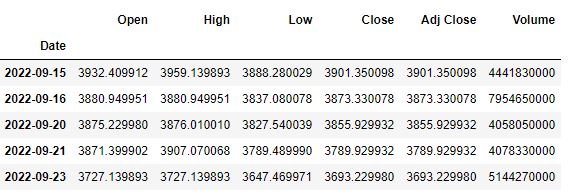
Let’s edit the benchmark data
benchmark_vector = np.array(df[‘Close’])
by creating our daily returns
benchmark_vector = np.diff(benchmark_vector)/benchmark_vector[1:]
benchmark_return = np.average(benchmark_vector)
benchmark_risk = np.std(benchmark_vector)
and modify our return and risk vectors
return_vector.append(benchmark_return)
risk_vector.append(benchmark_risk)
Let’s perform our portfolio analysis
portfolio_vector = np.array(df2[‘Close’])
Let’s iterate through the number of pre-defined scenarios
for i in range(number_of_scenarios):
#Create a random distribution that sums 1
# and is split by the number of stocks in the portfolio
random_distribution = np.random.dirichlet(np.ones(len(portfolio_)),size=1)
distrib_vector.append(random_distribution)
#Find the Closing Price for everyday of the portfolio
portfolio_matmul = np.matmul(random_distribution,portfolio_vector.T)

#Calculate the daily return
portfolio_matmul = np.diff(portfolio_matmul)/portfolio_matmul[:,1:]

#Select or Final Return and Risk
portfolio_return = np.average(portfolio_matmul, axis=1)
portfolio_risk = np.std(portfolio_matmul, axis=1)

#Add our Benchmark info to our lists
return_vector.append(portfolio_return[0])
risk_vector.append(portfolio_risk[0])
Let’s define the risk boundaries
delta_risk = 0.1
min_risk = np.min(risk_vector)
max_risk = risk_vector[0]*(1+delta_risk)
risk_gap = [min_risk, max_risk]
Let’s merge the portfolio return and risk
portfolio_array = np.column_stack((return_vector,risk_vector))[1:,]
and define the rule to create the best portfolio
If the criteria of min risk is satisfied then:
if np.where(((portfolio_array[:,1]<= max_risk)))[0].shape[0]>1:
min_risk_portfolio = np.where(((portfolio_array[:,1]<= max_risk)))[0]
best_portfolio_loc = portfolio_array[min_risk_portfolio]
max_loc = np.argmax(best_portfolio_loc[:,0])
best_portfolio = best_portfolio_loc[max_loc]
Otherwise, if the criteria of min risk is not satisfied, then:
else:
min_risk_portfolio = np.where(((portfolio_array[:,1]== np.min(risk_vector[1:]))))[0]
best_portfolio_loc = portfolio_array[min_risk_portfolio]
max_loc = np.argmax(best_portfolio_loc[:,0])
best_portfolio = best_portfolio_loc[max_loc]
The Visual Representation is
trade_days_per_year = 252
risk_gap = np.array(risk_gap)trade_days_per_year best_portfolio[0] = np.array(best_portfolio[0])trade_days_per_year
x = np.array(risk_vector)
y = np.array(return_vector)*trade_days_per_year
fig, ax = plt.subplots(figsize=(20, 15))
plt.rc(‘axes’, titlesize=14) # Controls Axes Title
plt.rc(‘axes’, labelsize=14) # Controls Axes Labels
plt.rc(‘xtick’, labelsize=14) # Controls x Tick Labels
plt.rc(‘ytick’, labelsize=14) # Controls y Tick Labels
plt.rc(‘legend’, fontsize=14) # Controls Legend Font
plt.rc(‘figure’, titlesize=14) # Controls Figure Title
ax.scatter(x, y, alpha=0.5,
linewidths=0.1,
edgecolors=’black’,
label=’Portfolio Scenarios’
)
ax.scatter(x[0],
y[0],
color=’red’,
linewidths=1,
edgecolors=’black’,
label=’Market Proxy Values’)
ax.scatter(best_portfolio[1],
best_portfolio[0],
color=’green’,
linewidths=1,
edgecolors=’black’,
label=’Best Performer’)
ax.axvspan(min_risk,
max_risk,
color=’red’,
alpha=0.08,
label=’Accepted Risk Zone’)
ax.set_ylabel(“Yearly Portfolio Average Return (%)”,fontsize=14)
ax.set_xlabel(“Yearly Portfolio Standard Deviation”,fontsize=14)
ax.axhline(y=0, color=’black’,alpha=0.5)
ax = plt.gca()
ax.legend(loc=0)
vals = ax.get_yticks()
ax.set_yticklabels([‘{:,.2%}’.format(x) for x in vals])
plt.savefig(‘risk_optimizer.png’, dpi=300)
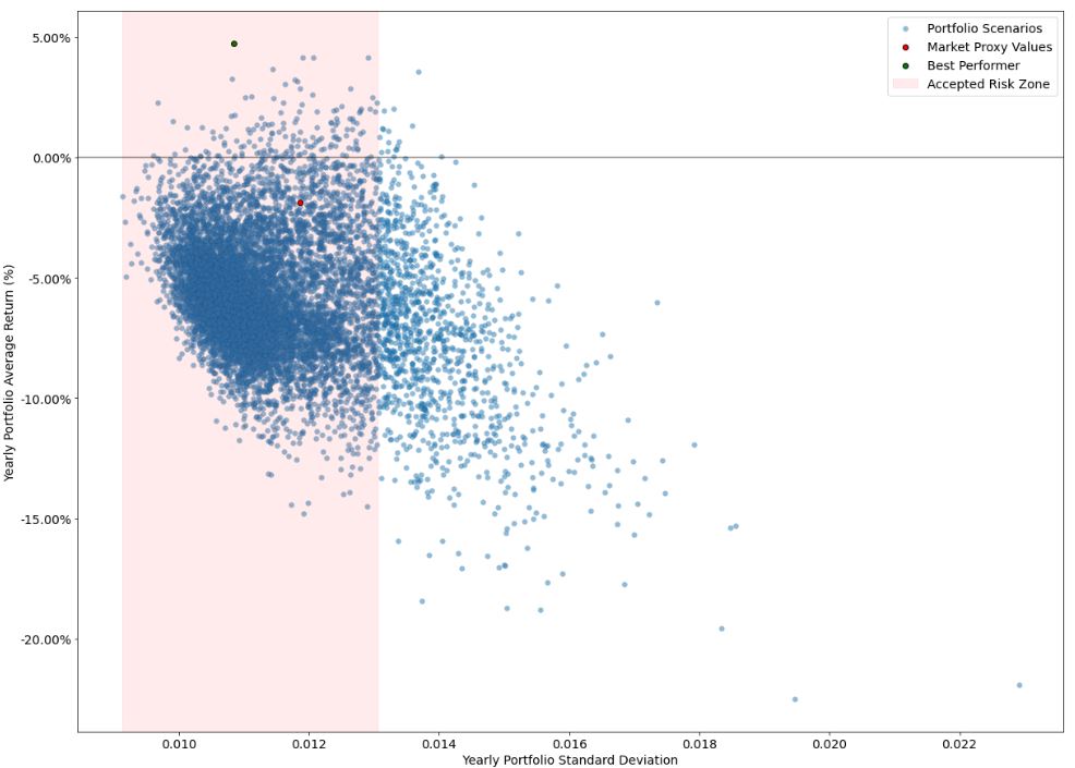
This plot shows the market performing (red dot) and then the maximum return at the minimum risk. That means if you would’ve held that portfolio between start and end date, you would’ve had a better portfolio than the market benchmark.
Let’s look at the output table of distributions
portfolio_loc = np.where((portfolio_array[:,0]==(best_portfolio[0]/trade_days_per_year))&(portfolio_array[:,1]==(best_portfolio[1])))[0][0]
best_distribution = distrib_vector[portfolio_loc][0].tolist()
d = {“Stock Name”: portfolio_, “Stock % in Portfolio”: best_distribution}
output = pd.DataFrame(d)
output = output.sort_values(by=[“Stock % in Portfolio”],ascending=False)
output= output.style.format({“Stock % in Portfolio”: “{:.2%}”})
output
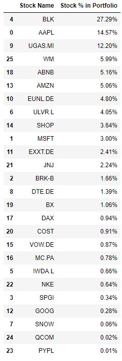
The above portfolio optimization script is the efficient way to assess whether investment goals and outcomes have been met.
Explore More


Leave a comment