The Qullamaggie’s TSLA Breakouts for Swing Traders

This project was inspired by the Qullamaggie’s breakout strategy for swing traders implemented as a simple stock scanner in Python. We will download the TSLA historical data from Yahoo finance.

Let’s set the working directory YOURPATH and import libraries

import os

os.chdir(‘YOURPATH’)

os. getcwd()

import numpy as np
import pandas as pd
import yfinance as yf

import seaborn as sns
import matplotlib.pyplot as plt
import matplotlib

Let’s define and call the following functions:

def trend_filter(prices: pd.core.series.Series,
growth_4_min: float = 25.,
growth_12_min: float = 50.,
growth_24_min: float = 80.) -> np.array:
”’
Take in a pandas series and output a binary array to indicate if a stock
fits the growth criteria (1) or not (0)
Parameters
———-
prices : pd.core.series.Series
The prices we are using to check for growth
growth_4_min : float, optional
The minimum 4 week growth. The default is 25
growth_12_min : float, optional
The minimum 12 week growth. The default is 50
growth_24_min : float, optional
The minimum 24 week growth. The default is 80
Returns
——-
np.array
A binary array showing the positions where the growth criteria is met
”’

growth_func = lambda x: 100*(x.values[-1]/x.min() - 1)

growth_4 = df['Close'].rolling(20).apply(growth_func) > growth_4_min
growth_12 = df['Close'].rolling(60).apply(growth_func) > growth_12_min
growth_24 = df['Close'].rolling(120).apply(growth_func) > growth_24_min

return np.where(
    growth_4 | growth_12 | growth_24,
    1,
    0,
)

if name == ‘main‘:

df = yf.download('TSLA')
df.loc[:, 'trend_filter'] = trend_filter(df['Close'])
df.dropna()

[*********************100%***********************]  1 of 1 completed

df_trending = df[df[‘trend_filter’] == 1]

def explicit_heat_smooth(prices: np.array,
t_end: float = 5.0) -> np.array:
”’
Smoothen out a time series using a explicit finite difference method.
Parameters
———-
prices : np.array
The price to smoothen
t_end : float
The time at which to terminate the smootheing (i.e. t = 2)
Returns
——-
P : np.array
The smoothened time-series
”’

k = 0.1 # Time spacing, must be < 1 for numerical stability

# Set up the initial condition
P = prices

t = 0
while t < t_end:
    # Solve the finite difference scheme for the next time-step
    P = k*(P[2:] + P[:-2]) + P[1:-1]*(1-2*k)

    # Add the fixed boundary conditions since the above solves the interior
    # points only
    P = np.hstack((
        np.array([prices[0]]),
        P,
        np.array([prices[-1]]),
    ))
    t += k

return P

def check_consolidation(prices: np.array,
perc_change_days: int,
perc_change_thresh: float,
check_days: int) -> int:
”’
Smoothen the time-series and check for consolidation, see the
docstring of find_consolidation for the parameters
”’

# Find the smoothed representation of the time series
prices = explicit_heat_smooth(prices)

# Perc change of the smoothed time series to perc_change_days days prior
perc_change = prices[perc_change_days:]/prices[:-perc_change_days] - 1

consolidating = np.where(np.abs(perc_change) < perc_change_thresh, 1, 0)

# Provided one entry in the last n days passes the consolidation check,
# we say that the financial instrument is in consolidation on the end day
if np.sum(consolidating[-check_days:]) > 0:
    return 1
else:
    return 0

def find_consolidation(prices: np.array,
days_to_smooth: int = 50,
perc_change_days: int = 5,
perc_change_thresh: float = 0.015,
check_days: int = 5) -> np.array:
”’
Return a binary array to indicate whether each of the data-points are
classed as consolidating or not
Parameters
———-
prices : np.array
The price time series to check for consolidation
days_to_smooth : int, optional
The length of the time-series to smoothen (days). The default is 50.
perc_change_days : int, optional
The days back to % change compare against (days). The default is 5.
perc_change_thresh : float, optional
The range trading % criteria for consolidation. The default is 0.015.
check_days : int, optional
This says the number of lookback days to check for any consolidation.
If any days in check_days back is consolidating, then the last data
point is said to be consolidating. The default is 5.
Returns
——-
res : np.array
The binary array indicating consolidation (1) or not (0)
”’

res = np.full(prices.shape, np.nan)

for idx in range(days_to_smooth, prices.shape[0]):
    res[idx] = check_consolidation(
        prices = prices[idx-days_to_smooth:idx],
        perc_change_days = perc_change_days,
        perc_change_thresh = perc_change_thresh,
        check_days = check_days,
    )

return res

if name == ‘main‘:

df = yf.download('TSLA')
df.loc[:, 'consolidating'] = find_consolidation(df['Close'].values)
df.dropna()

[*********************100%***********************]  1 of 1 completed

Let’s check the content of our data frame df

df.info()

class 'pandas.core.frame.DataFrame'>
DatetimeIndex: 3051 entries, 2010-06-29 to 2022-08-10
Data columns (total 9 columns):
 #   Column         Non-Null Count  Dtype  
---  ------         --------------  -----  
 0   Open           3051 non-null   float64
 1   High           3051 non-null   float64
 2   Low            3051 non-null   float64
 3   Close          3051 non-null   float64
 4   Adj Close      3051 non-null   float64
 5   Volume         3051 non-null   int64  
 6   consolidating  3001 non-null   float64
 7   trend_filter   3051 non-null   int32  
 8   filtered       3051 non-null   bool   
dtypes: bool(1), float64(6), int32(1), int64(1)
memory usage: 205.6 KB

Let’s look at the date index

df.index = pd.DatetimeIndex(data=df.index, tz=’US/Eastern’) # naive–> aware

df.index

DatetimeIndex(['2010-06-29 00:00:00-04:00', '2010-06-30 00:00:00-04:00',
               '2010-07-01 00:00:00-04:00', '2010-07-02 00:00:00-04:00',
               '2010-07-06 00:00:00-04:00', '2010-07-07 00:00:00-04:00',
               '2010-07-08 00:00:00-04:00', '2010-07-09 00:00:00-04:00',
               '2010-07-12 00:00:00-04:00', '2010-07-13 00:00:00-04:00',
               ...
               '2022-07-28 00:00:00-04:00', '2022-07-29 00:00:00-04:00',
               '2022-08-01 00:00:00-04:00', '2022-08-02 00:00:00-04:00',
               '2022-08-03 00:00:00-04:00', '2022-08-04 00:00:00-04:00',
               '2022-08-05 00:00:00-04:00', '2022-08-08 00:00:00-04:00',
               '2022-08-09 00:00:00-04:00', '2022-08-10 00:00:00-04:00'],
              dtype='datetime64[ns, US/Eastern]', name='Date', length=3051, freq=None)

dft = pd.DataFrame({‘DateTime’: df.index})

dft.DateTime

0      2010-06-29 00:00:00-04:00
1      2010-06-30 00:00:00-04:00
2      2010-07-01 00:00:00-04:00
3      2010-07-02 00:00:00-04:00
4      2010-07-06 00:00:00-04:00
                  ...           
3046   2022-08-04 00:00:00-04:00
3047   2022-08-05 00:00:00-04:00
3048   2022-08-08 00:00:00-04:00
3049   2022-08-09 00:00:00-04:00
3050   2022-08-10 00:00:00-04:00
Name: DateTime, Length: 3051, dtype: datetime64[ns, US/Eastern]

Selecting rows based on condition
df1 = df[df[‘filtered’] > 0]
df0 = df[df[‘filtered’] < 1]

dft1 = pd.DataFrame({‘DateTime’: df1.index})
dft0 = pd.DataFrame({‘DateTime’: df0.index})

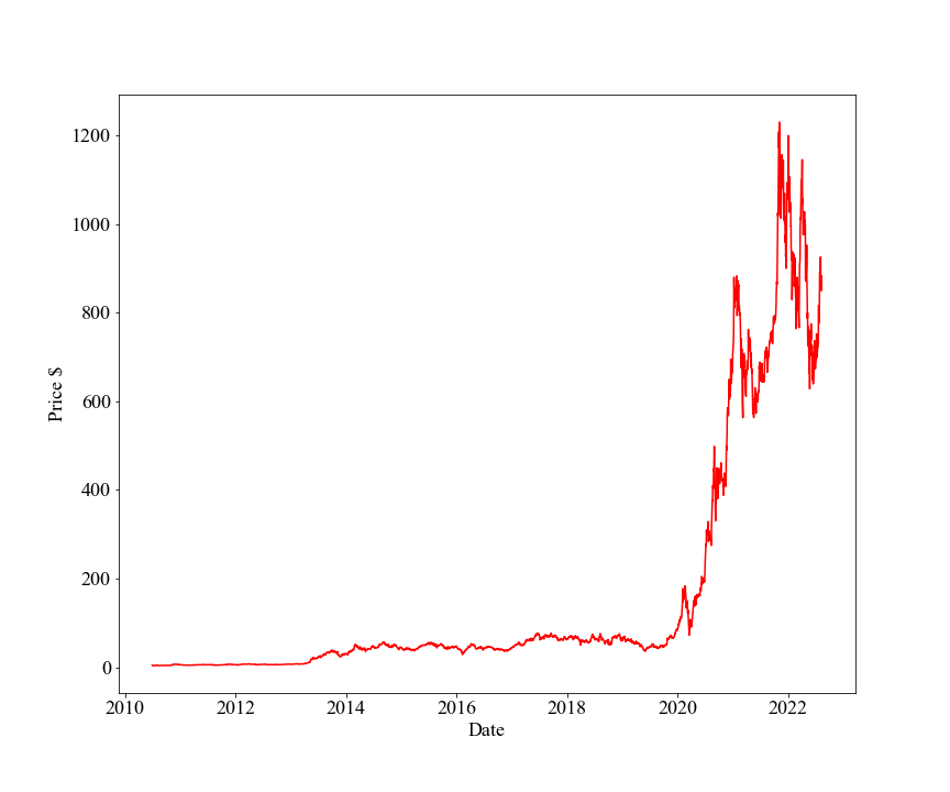
Let’s plot the TSLA stock price 2010-2022

plt.figure(figsize=(12,10))
matplotlib.rcParams.update({‘font.size’: 18})
import matplotlib.pyplot as plt
plt.plot(dft.DateTime,df.Close, ‘r’)
plt.xlabel(“Date”)
plt.ylabel(“Price $”)
plt.savefig(‘tslaprice.png’)

Let’s display the original close price (red) vs filtered data or breakouts (green) as the following composite scatter plot

plt.figure(figsize=(12,10))
scal=5e5
plt.scatter(df0.index, df0[“Close”],color=’red’,s=df0[“Volume”]/scal,alpha=0.4)
plt.scatter(df1.index, df1[“Close”],color=’green’,s=df1[“Volume”]/scal,alpha=0.4)
plt.xlabel(“Date”)
plt.ylabel(“Price $”)

plt.legend([“Close” , “Filtered”], facecolor=’bisque’,
loc=’upper center’, bbox_to_anchor=(0.5, -0.08),
ncol=2)
plt.grid()
plt.show()
plt.savefig(‘tslapriceswingfilter.png’)

This is done by using the following breakout parameters:

Time-series days to smoothen = 50 days
How many days back to percentage check = 5 (i.e. percentage change of the recent day to 5 days ago, to see if it’s rangebound).
The threshold % to define a rangebound data-point = 1.5%
The number of days to check for consolidation = 5

The above plot shows the “filtered” price where we observe consolidation that meets the growth criteria at a given date/time. This scanner is very simple and efficient in that it can be applied to a 1000’s of stocks to identify potential consolidation/breakout patterns of interest to swing traders.

My scanning process and scans

Regarding Qullamaggies’s video named ‘My scanning process and scans’