Applications of ML/AI in HR – Predicting Employee Attrition

AI for Human Resources: Predict attrition of your valuable employees using Machine Learning

An organization’s human resources (HR) function deals with the most valuable asset: people. Human resources play an important role in the success of a business. Human resources face many challenges and AI can help automate and solve some of these challenges.

Recently, the HR role has largely expanded into a driver of value to be in a position to strategize for recruitment, engagement, and retention.

A critical arm of artificial intelligence (AI), machine learning (ML) is making strides in every area of HR.

On the other hand, AI may face a lot of challenges in HR like Low volume of historical data, Privacy concerns of employees, and low priority for AI projects

Managing employees means gathering (big) data in a host of areas – employee attitudes and feelings, qualification verification, employee approach towards policies, compensation management, etc. Here’s where ML/AI comes in via HR analytics in the following areas:

• Smarter candidate identification and applicant tracking

• Smart predictions about employee turnover

• Smart predictions about job success

For example, let’s look at the

HR DATA TO PREDICT WHICH EMPLOYEES ARE LIKELY TO LEAVE.

The Kaggle reference is

HR Analytics: Job Change of Data Scientists

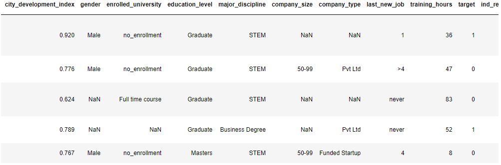
The csv files of interest are aug_train and aug_test.

These two tables contain several columns (model features).

Features:

• enrollee_id : Unique ID for candidate
• city: City code
• city_ development _index : Developement index of the city (scaled)
• gender: Gender of candidate
• relevent_experience: Relevant experience of candidate
• enrolled_university: Type of University course enrolled if any
• education_level: Education level of candidate
• major_discipline :Education major discipline of candidate
• experience: Candidate total experience in years
• company_size: No of employees in current employer’s company
• company_type : Type of current employer
• lastnewjob: Difference in years between previous job and current job
• training_hours: training hours completed
• target: 0 – Not looking for job change, 1 – Looking for a job change

Context and Content

A company which is active in Big Data and Data Science wants to hire data scientists among people who successfully pass some courses which conduct by the company. Many people signup for their training. Company wants to know which of these candidates are really wants to work for the company after training or looking for a new employment because it helps to reduce the cost and time as well as the quality of training or planning the courses and categorization of candidates. Information related to demographics, education, experience are in hands from candidates signup and enrollment.

This dataset designed to understand the factors that lead a person to leave current job for HR researches too. By model(s) that uses the current credentials,demographics,experience data you will predict the probability of a candidate to look for a new job or will work for the company, as well as interpreting affected factors on employee decision.

The whole data divided to train and test . Target isn’t included in test but the test target values data file is in hands for related tasks. 

Note:

• The dataset is imbalanced.
• Most features are categorical (Nominal, Ordinal, Binary), some with high cardinality.
• Missing imputation can be a part of your pipeline as well.

Objectives

• Predict the probability of a candidate will work for the company
• Interpret model(s) such a way that illustrate which features affect candidate decision

The dataset was prepared for ML tasks by TheAnalyticsLab by implementing the following steps:

* Convert target to integer
* Create dataframe with cities and a rank based on the city development index
* Download innovation index values of metropolitan areas and prepare for matching to cities
* Create dataframe with city id and city name matched on index ranks and add city name to our data
* Convert relevent_experience to a dummy
* Create a numeric version of experience

The final output file df_prepared.csv is stored on the Azure blob storage.

XGB Prediction

We are going to follow the HR analytics journey of Meta (it’s all about speed) and Aki (it’s all about accuracy) using the above file. The task at hand is to predict which employees might leave the company. Following Jurriaan Nagelkerke, we will visualise the business value of Meta/Aki predictive models using the modelplotpy package.

Let’s set the working directory

import os

os.chdir(‘YOURPATH’)

os. getcwd()

and import the Python packages and settings

from sklearn.impute import SimpleImputer
from sklearn.pipeline import Pipeline
from sklearn.preprocessing import StandardScaler, OneHotEncoder
from sklearn.compose import ColumnTransformer
from sklearn.model_selection import train_test_split
from sklearn import metrics
import xgboost as xgb
from sklearn.model_selection import StratifiedKFold
from sklearn.model_selection import cross_val_score
from sklearn.model_selection import GridSearchCV
from sklearn.metrics import roc_curve

import pandas as pd

import warnings
warnings.filterwarnings(action= ‘ignore’)
import pandas as pd
import numpy as np
from sklearn.impute import SimpleImputer
from sklearn.pipeline import Pipeline
from sklearn.preprocessing import StandardScaler, OneHotEncoder
from sklearn.compose import ColumnTransformer
from sklearn.model_selection import train_test_split
import xgboost as xgb
from sklearn.model_selection import StratifiedKFold
from sklearn.model_selection import cross_val_score
import joblib

import modelplotpy as mp

import matplotlib.pyplot as plt

%matplotlib inline

Loading the data:
df_prep = pd.read_csv(‘https://bhciaaablob.blob.core.windows.net/featurenegineeringfiles/df_prepared.csv’)
df = df_prep.drop(columns=[‘Unnamed: 0′,’city’, ‘experience’, ‘enrollee_id’])
df.head()

Let’s define the target vector y
y = df[‘target’]

Creating a dataset without the DV:
X = df.drop(‘target’, axis = 1)

Let’s split X and y into training and testing sets with test_size=0.25
X_train, X_test, y_train, y_test = train_test_split(
X, y, test_size=0.25, stratify=y, random_state=1121218
)

Create an object with the column labels of only the categorical features and one with only the numeric features:
categorical_features = X.select_dtypes(exclude=”number”).columns.tolist()
numeric_features = X.select_dtypes(include=”number”).columns.tolist()

Create the categorical pipeline, for the categorical variables Meta imputes the missing values with a constant value and we encode them with One-Hot encoding:
categorical_pipeline = Pipeline(
steps=[
(“impute”, SimpleImputer(strategy= ‘constant’, fill_value= ‘unknown’)),
(“one-hot”, OneHotEncoder(handle_unknown=”ignore”, sparse=False))
]
)

Create the numeric pipeline, for the numeric variables Meta imputes the missings with the mean of the column and standardize them, so that the features have a mean of 0 and a variance of 1:
numeric_pipeline = Pipeline(
steps=[(“impute”, SimpleImputer(strategy=”mean”)),
(“scale”, StandardScaler())]
)

Combining the two pipelines with a column transformer:
full_processor = ColumnTransformer(transformers=[
(“numeric”, numeric_pipeline, numeric_features),
(“categorical”, categorical_pipeline, categorical_features),
]
)

Meta instantiates the XGBClassifier, since we are dealing with a classification task:
xgb_cl = xgb.XGBClassifier(eval_metric=’logloss’, seed=7)

Create XGBoost pipeline:
xgb_pipeline = Pipeline(steps=[
(‘preprocess’, full_processor),
(‘model’, xgb_cl)
])

Evaluate the model with the use of cv:
cv = StratifiedKFold(n_splits=5, shuffle=True, random_state=7) #, shuffle=True with or without shuffle??
scores = cross_val_score(xgb_pipeline, X_train, y_train, cv=cv, scoring = ‘roc_auc’)
print(“roc_auc = %f (%f)” % (scores.mean(), scores.std()))

roc_auc = 0.791519 (0.004802)

Let’s look at the default hyperparameters of the XGBoost:
xgb_cl

XGBClassifier(base_score=None, booster=None, callbacks=None,
              colsample_bylevel=None, colsample_bynode=None,
              colsample_bytree=None, early_stopping_rounds=None,
              enable_categorical=False, eval_metric='logloss', gamma=None,
              gpu_id=None, grow_policy=None, importance_type=None,
              interaction_constraints=None, learning_rate=None, max_bin=None,
              max_cat_to_onehot=None, max_delta_step=None, max_depth=None,
              max_leaves=None, min_child_weight=None, missing=nan,
              monotone_constraints=None, n_estimators=100, n_jobs=None,
              num_parallel_tree=None, predictor=None, random_state=None,
              reg_alpha=None, reg_lambda=None, ...)

Let’s train the Meta’s default XGBoost pipeline:
xgb_pipeline.fit(X_train, y_train)

Load the models:
upload_pipe_meta = joblib.load(‘pipe_meta.joblib’)

Use it to make the same predictions:
print(upload_pipe_meta.predict(X_train))

[0 0 1 ... 0 0 1]

In the code below Aki separates the target from the features, creates train/test datasets and the pipelines to prep the features.

By creating the categorical pipeline, Aki imputes the missing categorical values with a constant value. We encode them with One-Hot encoding:
categorical_pipeline = Pipeline(
steps=[
(“impute”, SimpleImputer(strategy= ‘constant’, fill_value= ‘unknown’)),
(“one-hot”, OneHotEncoder(handle_unknown=”ignore”, sparse=False))
]
)

Combining the two pipelines with a column transformer:
full_processor = ColumnTransformer(transformers=[
(“numeric”, numeric_pipeline, numeric_features),
(“categorical”, categorical_pipeline, categorical_features),
]
)

We instantiate the XGBClassifier:
xgb_cl = xgb.XGBClassifier(eval_metric=’logloss’, seed=7)

Create XGBoost pipeline:
xgb_pipeline = Pipeline(steps=[
(‘preprocess’, full_processor),
(‘model’, xgb_cl)
])

We evaluate the model using cv:
cv = StratifiedKFold(n_splits=5, shuffle=True, random_state=7) #, shuffle=True with or without shuffle??
scores = cross_val_score(xgb_pipeline, X_train, y_train, cv=cv, scoring = ‘roc_auc’)
print(“roc_auc = %f (%f)” % (scores.mean(), scores.std()))

roc_auc = 0.791519 (0.004802)

Let’s introduce the function

def print_results_gridsearch(gridsearch, list_param1, list_param2, name_param1, name_param2):

# Checking the results from each run in the gridsearch:
means = gridsearch.cv_results_[‘mean_test_score’]
stds = gridsearch.cv_results_[‘std_test_score’]
params = gridsearch.cv_results_[‘params’]
print(“The results from each run in the gridsearch:”)
for mean, stdev, param in zip(means, stds, params):
print(“roc_auc = %f (%f) with: %r” % (mean, stdev, param))

#Visualizing the results from each run in the gridsearch:
scores = np.array(means).reshape(len(list_param1), len(list_param2))
for i, value in enumerate(list_param1):
plt.plot(list_param2, scores[i], label= str(name_param1) + ‘: ‘ + str(value))
plt.legend()
plt.xlabel(str(name_param2))
plt.ylabel(‘ROC AUC’)
plt.show()

# Checking the best performing model:
print(“\n”)
print(“Best model: roc_auc = %f using %s” % (gridsearch.best_score_, gridsearch.best_params_))

Hyperparameter Optimization (HPO)

Step 1: Searching for the optimum parameters for the learning rate and the number of estimators:

Defining the parameter grid to be used in GridSearch:
param_grid = {“model__subsample”: [0.8], “model__colsample_bytree”: [0.8]
, “model__learning_rate”: [0.0001, 0.001, 0.01, 0.1, 0.2, 0.3]
, “model__n_estimators”: range(50,500,50)
}

Instantiate the Grid Search:
cv = StratifiedKFold(n_splits=5, shuffle=True, random_state=7)
grid_cv1 = GridSearchCV(xgb_pipeline
, param_grid
, n_jobs= -1
, cv = cv
, scoring=”roc_auc”)

Fit
_ = grid_cv1.fit(X_train, y_train)

Checking the results from each run in the gridsearch:
print_results_gridsearch(gridsearch=grid_cv1, list_param1 = param_grid[“model__learning_rate”], list_param2 = param_grid[“model__n_estimators”]
, name_param1 = ‘learning_rate’ , name_param2 = ‘n_estimators’)

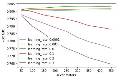
Best model: roc_auc = 0.803255 using {'model__colsample_bytree': 0.8, 'model__learning_rate': 0.01, 'model__n_estimators': 350, 'model__subsample': 0.8}

Step 2: Searching for the optimum parameters for max_depth and min_child_weight:

Defining the parameter grid to be used in GridSearch:
param_grid = {“model__subsample”: [0.8], “model__colsample_bytree”: [0.8], “model__learning_rate”: [0.01], “model__n_estimators”: [250]
, ‘model__max_depth’: range(3,10,2)
, ‘model__min_child_weight’: range(1,6,2)
}

Instantiate the Grid Search:
cv = StratifiedKFold(n_splits=5, shuffle=True, random_state=7)
grid_cv2 = GridSearchCV(xgb_pipeline
, param_grid
, n_jobs=-1
, cv=cv
, scoring=”roc_auc”)

Fit
_ = grid_cv2.fit(X_train, y_train)

Checking the results from each run in the gridsearch:
print_results_gridsearch(gridsearch=grid_cv2, list_param1 = param_grid[“model__max_depth”], list_param2 = param_grid[“model__min_child_weight”]
, name_param1 = ‘max_depth’ , name_param2 = ‘min_child_weight’)

Best model: roc_auc = 0.803567 using {'model__colsample_bytree': 0.8, 'model__learning_rate': 0.01, 'model__max_depth': 5, 'model__min_child_weight': 1, 'model__n_estimators': 250, 'model__subsample': 0.8}

Step 3: Searching for the optimum parameters for subsample and colsample_bytree:

Defining the parameter grid to be used in GridSearch:
param_grid = {“model__learning_rate”: [0.01], “model__n_estimators”: [250], ‘model__max_depth’: [5], ‘model__min_child_weight’: [1]
, ‘model__subsample’:[i/10.0 for i in range(4,10)]
, ‘model__colsample_bytree’:[i/10.0 for i in range(4,10)]
}

Instantiate the Grid Search:
cv = StratifiedKFold(n_splits=5, shuffle=True, random_state=7)
grid_cv3 = GridSearchCV(xgb_pipeline
, param_grid
, n_jobs=-1
, cv=cv
, scoring=”roc_auc”)

Fit
_ = grid_cv3.fit(X_train, y_train)

Checking the results from each run in the gridsearch:
print_results_gridsearch(gridsearch=grid_cv3, list_param1 = param_grid[“model__subsample”], list_param2 = param_grid[“model__colsample_bytree”]
, name_param1 = ‘subsample’ , name_param2 = ‘colsample_bytree’)

Best model: roc_auc = 0.803910 using {'model__colsample_bytree': 0.8, 'model__learning_rate': 0.01, 'model__max_depth': 5, 'model__min_child_weight': 1, 'model__n_estimators': 250, 'model__subsample': 0.5}

Step 4: Searching for the optimum parameters for gamma and lambda:

Defining the parameter grid to be used in GridSearch:
param_grid = {“model__learning_rate”: [0.01], “model__n_estimators”: [250], ‘model__max_depth’: [5], ‘model__min_child_weight’: [1], ‘model__subsample’:[0.5], ‘model__colsample_bytree’:[0.9]
, “model__gamma”: [i/10.0 for i in range(0,6)]
, “model__reg_lambda”: [0, 0.5, 1, 1.5, 2, 3, 4.5]
}

Instantiate the Grid Search:
cv = StratifiedKFold(n_splits=5, shuffle=True, random_state=7)
grid_cv4 = GridSearchCV(xgb_pipeline
, param_grid
, n_jobs=-1
, cv=cv
, scoring=”roc_auc”)

Fit
_ = grid_cv4.fit(X_train, y_train)

Checking the results from each run in the gridsearch:
print_results_gridsearch(gridsearch=grid_cv4, list_param1 = param_grid[“model__gamma”], list_param2 = param_grid[“model__reg_lambda”]
, name_param1 = ‘Gamma’ , name_param2 = ‘Lambda’)

Best model: roc_auc = 0.803900 using {'model__colsample_bytree': 0.9, 'model__gamma': 0.5, 'model__learning_rate': 0.01, 'model__max_depth': 5, 'model__min_child_weight': 1, 'model__n_estimators': 250, 'model__reg_lambda': 1.5, 'model__subsample': 0.5}

Let’s print out the best hyperparameters (output of HPO)

grid_cv4.best_params_

{'model__colsample_bytree': 0.9,
 'model__gamma': 0.5,
 'model__learning_rate': 0.01,
 'model__max_depth': 5,
 'model__min_child_weight': 1,
 'model__n_estimators': 250,
 'model__reg_lambda': 1.5,
 'model__subsample': 0.5}

Let’s predict with Aki’s final XGBoost using the best parameters resulting from the GridSearch:
y_pred_aki = grid_cv4.predict(X_test)
y_pred_prob_aki = grid_cv4.predict_proba(X_test)[::,1]

Evaluate:
print(“roc_auc_score:”,metrics.roc_auc_score(y_test, y_pred_aki))

roc_auc_score: 0.7131171709492959

Let’s fit the Meta’s default XGBoost pipeline:
xgb_pipeline.fit(X_train, y_train)

Predict:
y_pred_meta = xgb_pipeline.predict(X_test)
y_pred_prob_meta = xgb_pipeline.predict_proba(X_test)[::,1]

Evaluate:
print(“roc_auc_score:”,metrics.roc_auc_score(y_test, y_pred_meta))

roc_auc_score: 0.6993045967695355

Let’s compute False postive rate, and True positive rate
fpr1 , tpr1, thresholds1 = roc_curve(y_test, y_pred_prob_aki)
fpr2 , tpr2, thresholds2 = roc_curve(y_test, y_pred_prob_meta)

Calculate Area under the curve to display on the plot
roc_auc_aki = metrics.roc_auc_score(y_test, y_pred_aki)
roc_auc_meta = metrics.roc_auc_score(y_test, y_pred_meta)

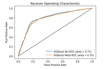
Now, plot the computed values
plt.plot([0,1],[0,1], ‘k–‘)
plt.plot(fpr1, tpr1, label= ‘%s ROC (area = %0.2f)’ % (“XGBoost Aki”, roc_auc_aki)) #”XGBoost Aki”)
plt.plot(fpr2, tpr2, label= ‘%s ROC (area = %0.2f)’ % (“XGBoost Meta”, roc_auc_meta)) #label= “XGBoost Meta”)
plt.legend()
plt.xlabel(‘False Positive Rate’)
plt.ylabel(‘True Positive Rate’)
plt.title(‘Receiver Operating Characteristic’)
plt.show()

Saving Aki’s final XGBoost pipeline:
best_pipe_aki = grid_cv4.best_estimator_
joblib.dump(best_pipe_aki, ‘best_pipe_aki.joblib’)

['best_pipe_aki.joblib']

Testing if Aki’s model is correctly saved:

Load the models:
upload_pipe_aki = joblib.load(‘best_pipe_aki.joblib’)

Use it to make the same predictions:
print(upload_pipe_aki.predict(X_test))

[0 1 0 ... 0 1 0]

Model Visualizations

Let’s assess the business value of the above predictive models using modelplotpy.

Let’s import 2 model pipelines
xgb_meta = joblib.load(‘pipe_meta.joblib’)
xgb_aki = joblib.load(‘best_pipe_aki.joblib’)

and transform train/test data generated with prepare_scores_and_deciles into aggregated data for chosen plotting scope

import modelplotpy as mp
obj = mp.modelplotpy(feature_data = [X_train, X_test]
, label_data = [y_train, y_test]
, dataset_labels = [‘train data’, ‘test data’]
, models = [xgb_meta, xgb_aki]
, model_labels = [‘Metas XGB', 'Akis XGB’]
)

ps = obj.plotting_scope(scope=’compare_models’,select_dataset_label = [‘test data’],select_targetclass=[1])

compare models

Let’s plot the cumulative gains plot and annotate the plot at decile = 3

_ = mp.plot_cumgains(ps, highlight_ntile = 3)

When we select 30% with the highest probability according to model Aki`s XGB, this selection holds 69% of all 1 cases in dataset test data.
When we select 30% with the highest probability according to model Meta`s XGB, this selection holds 66% of all 1 cases in dataset test data.

The cumulative gains plot visualises the percentage of the target class members you have selected if you would decide to select up until decile X. We can see that the Aki’s parameter tuning resulted in a slightly better model in that it is targeting a larger number of the actually leaving employees than that the Meta’s XGB.

Let’s plot the cumulative lift plot and annotate the plot at decile = 3
_ = mp.plot_cumlift(ps, highlight_ntile = 3)

When we select 30% with the highest probability according to model Aki`s XGB in dataset test data, this selection for target class 1 is 2.31 times than selecting without a model.
When we select 30% with the highest probability according to model Meta`s XGB in dataset test data, this selection for target class 1 is 2.22 times than selecting without a model.

The lift plot only has one reference line: the ‘random model’. With a random model we mean that each observation gets a random number and all cases are devided into deciles based on these random numbers. If 50% of your data belongs to the target class of interest, a perfect model would only do twice as good (lift: 2) as a random selection. 

We can see that both models more than double the quality of the selection, when compared to randomly selecting 30% of all employees for the employee retention program.

Let’s plot the response plot and annotate the plot at decile = 3
_ = mp.plot_response(ps, highlight_ntile = 3)

For the Aki’s and Meta models, the first three deciles consist of >50% and < 50% of actual leavers, respectively.

Let’s plot the cumulative response plot and annotate the plot at decile = 3
_ = mp.plot_cumresponse(ps, highlight_ntile = 3)

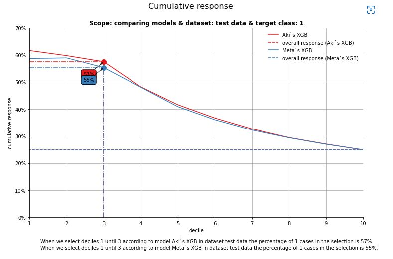
By selecting up until the third decile based on 2 models, the expected % of employees that is planning to leave is 55 and 57 % for the Meta and Aki models, respectively.

Conclusions

The aim of HR analytics and ML/AI is to provide HR managers with a better insight into their human resource strategies. With this data at the ready, it’s easier to pinpoint weaknesses in your recruiting methods and, subsequently, make necessary improvements. The HR professionals can use HR ML/AI to address the following issues:

• Your employee turnover rate
• The percentage of that turnover that’s a regrettable loss
• The experience and satisfaction of candidates during the recruitment process
• On the balance of probabilities, which employees will leave your organization within a year.

This article demonstrates that ML models can extract info from existing data to determine patterns and forecast future outcomes. These models are invaluable for adopting a more strategic and data-driven approach to HR. It has been shown that the above visual representations of ML models are essential for making valuable HR business decisions. 

Data-driven workforce decisions have a crucial influence on customer satisfaction and retention, especially when employees come into regular contact with customers. Knowing when employees are most likely to have a slump in productivity, fall ill, or quit, helps each department prepare for any and all of these eventualities.