Algorithmic Testing Stock Portfolios to Optimize the Risk/Reward Ratio

Investors can optimize their stock portfolio by invoking backtesting within the realm of algorithmic trading. The goal is to optimize the specific portfolio by maximizing returns and the Sharpe ratio.

The workflow in Python consists of the following steps:

• Import/install relevant libraries
• Define the stock portfolio & time interval
• Download historical data from Yfinance
• Apply the MVA strategy function to stock data
• Calculate cumulative returns and the annual Sharpe ratio
• Plot cumulative returns of individual stocks and the portfolio return

Let’s set the working directory YOURPATH

import os

os.chdir(‘YOURPATH’)

and import/install the following libraries

!pip install nsepy

import warnings
warnings.filterwarnings(‘ignore’)

import numpy as np
import pandas as pd
from datetime import datetime as dt
import yfinance as yf
import nsepy
from statistics import mean

Let’s define the following functions

Get daily data from Yfinance

def get_daily_data(symbol, start, end):
data = yf.download(tickers=symbol, start=start, end=end)
return data

MVA strategy on close price data

def ma(data,ma1,ma2):
# calculating moving averages
data[‘ma_short’] = data[‘Close’].ewm(span=ma1).mean().shift()
data[‘ma_long’] = data[‘Close’].ewm(span=ma2).mean().shift()

# creating positions
# data["position"] = [0]*len(data)
data['position'] = np.where(data["ma_short"] > data["ma_long"], 1, 0)    
data["strategy_returns"] = data["bnh_returns"] * data["position"]

# returning strategy returns
return data["strategy_returns"]

Cumulative returns function

def get_cumulative_return(df):
return list(df.cumsum())[-1]

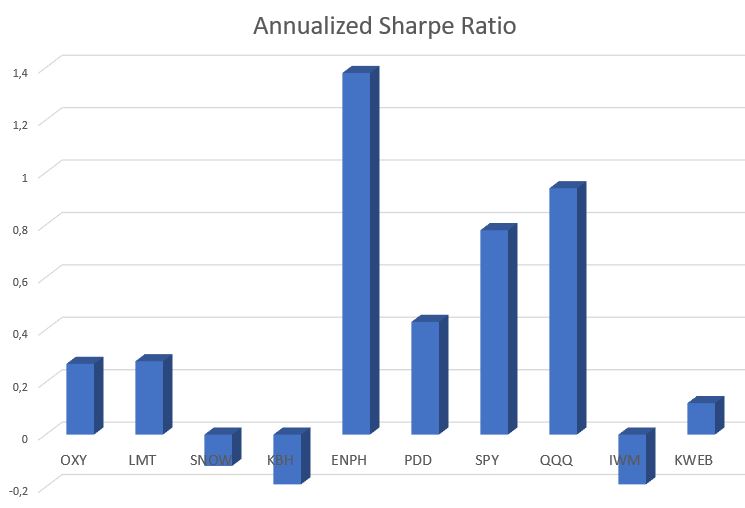
Annual Sharpe ratio function

def get_annualized_sharpe_ratio(df):
return 252**(1/2) * (df.mean() / df.std())

Let’s define the backtesting parameters
days = 2000
end = dt.today()
start = end – pd.Timedelta(days=days)

and the stock portfolio
portfolio_stocks = [“OXY”,”LMT”,”SNOW”,”KBH”,”ENPH”,”PDD”,”SPY”,”QQQ”,”IWM”,”KWEB”,]

based on the available market research studies, technical analysis, updates, market trends, and stock screeners.

Let’s define a data frame to store portfolio returns
portfolio_strategy_returns = pd.DataFrame()
portfolio_bnh_returns = pd.DataFrame()

Buy and hold returns for individual stocs
bnh_stock_returns = []
bnh_stock_sharpe = []

iterating over stocks in the portfolio
for stock in portfolio_stocks:
data = get_daily_data(stock, start, end)

# Calculating daily returns
data["bnh_returns"] = np.log(data["Close"]/data["Close"].shift())

portfolio_strategy_returns[stock] = ma(data,ma1 = 3, ma2 = 8)

bnh_stock_returns.append(get_cumulative_return(data["strategy_returns"]))
bnh_stock_sharpe.append(get_annualized_sharpe_ratio(data["strategy_returns"]))

[*********************100%***********************]  1 of 1 completed
[*********************100%***********************]  1 of 1 completed
[*********************100%***********************]  1 of 1 completed
[*********************100%***********************]  1 of 1 completed
[*********************100%***********************]  1 of 1 completed
[*********************100%***********************]  1 of 1 completed
[*********************100%***********************]  1 of 1 completed
[*********************100%***********************]  1 of 1 completed
[*********************100%***********************]  1 of 1 completed
[*********************100%***********************]  1 of 1 completed

print(“\nSTRATEGY RETURNS ON PORTFOLIO”)
portfolio_strategy_returns[“Portfolio_rets”] = portfolio_strategy_returns.mean(axis=1)
portfolio_strategy_returns.round(decimals = 4).tail(10)

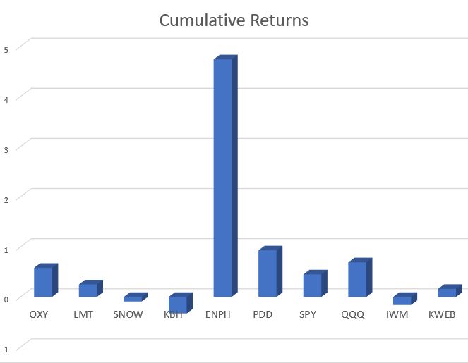
perf = pd.DataFrame(index=portfolio_stocks,columns=[“Cumulative returns”,”Annualized Sharpe Ratio”])

for i,stock in enumerate(portfolio_stocks):
cum_ret = bnh_stock_returns[i]
anu_shp = bnh_stock_sharpe[i]
perf.loc[stock] = [cum_ret,anu_shp]

perf

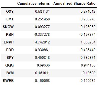
perf.mean()

Cumulative returns         0.722194
Annualized Sharpe Ratio    0.369893
dtype: float64

print(“Cumulative returns MA Strategy :”,get_cumulative_return(portfolio_strategy_returns[“Portfolio_rets”]))
print(“Annualized sharpe ratio MA Strategy :”,get_annualized_sharpe_ratio(portfolio_strategy_returns[“Portfolio_rets”]))
print(“\n”)

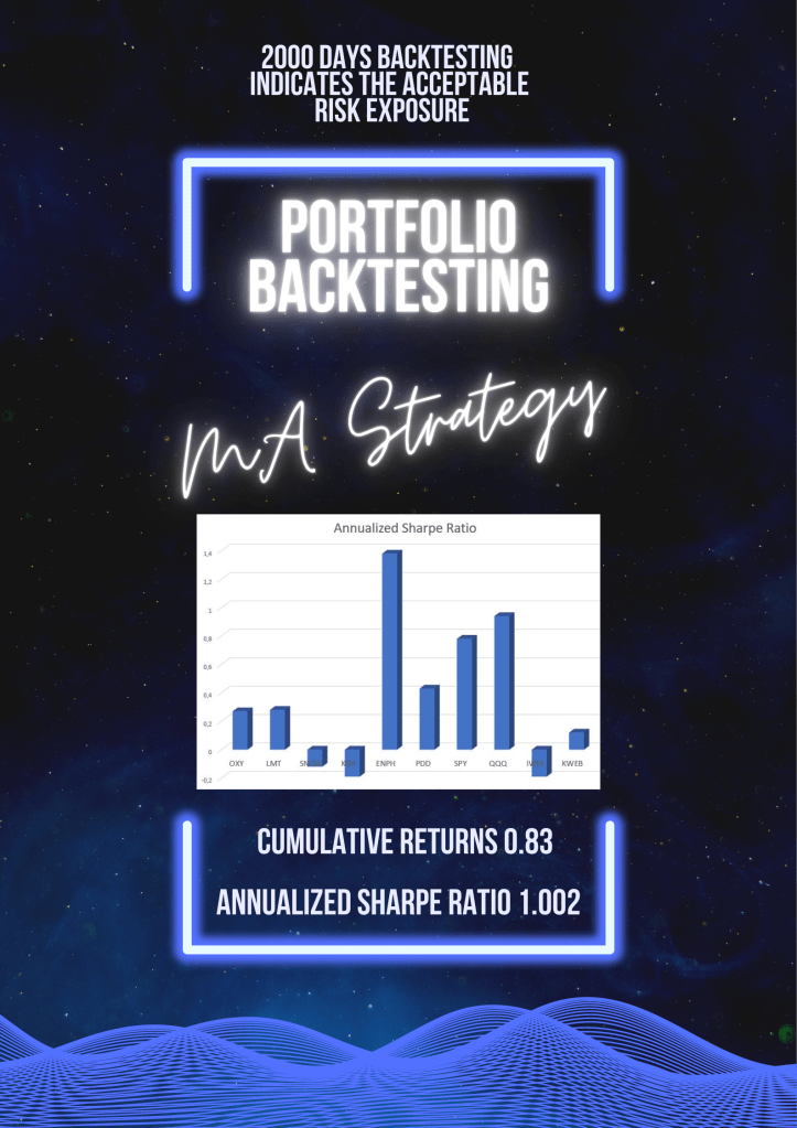
Cumulative returns MA Strategy                  : 0.832610455484652
Annualized sharpe ratio MA Strategy             : 1.0024619067938556

import matplotlib.pyplot as plt
colors = [‘tab:cyan’,’tab:purple’,’tab:pink’,’tab:orange’,’tab:blue’,’tab:green’,’tab:gray’,’tab:olive’,’tab:brown’,’tab:red’,”k”]
portfolio_strategy_returns.cumsum().plot(figsize=(20,10), title=”MOVING AVERAGES STRATEGY CUMULATIVE RETURNS”, color=colors)
plt.savefig(‘portfolioreturnspup.png’)

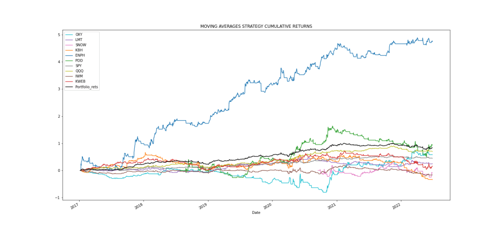
The plot shows that the portfolio has almost no variation as compared to the individual stock performance. The Sharpe ratio of 1.0024 indicates the acceptable risk exposure.

Infographic