Operating rooms (ORs) are some of the most valuable hospital assets, generating a large part of hospital revenue. For efficient utilization of ORs, accurate schedules of assigned block time and sequences of patient cases need to be made [1]. Statistical models have been developed using datasets to predict daily surgical volumes weeks in advance. The quest was motivated by the need to make real-time adjustments to staff capacity and reallocation of the OR block time based on predicted future demand.

Following previous studies [3,4], we focus on the VUMC dataset for evaluation of our statistical models. The dataset represents a 48-week surgery schedule for VUMC recorded from October 10, 2011 to September 14, 2012.
Our method consists of the ANOVA null-hypothesis test for the total number of surgeries to see if these variables change from day to day with 99% confidence. The null hypothesis H0 is the statement that the total number of surgeries does not depend upon the weekday (DOW). The alternative hypothesis states that the total number of surgeries does vary from day to day.
Next, the Ordinary Least Squares (OLS) linear regression formula [3,4] is applied to our target variable Actual Surgery as a function of 28 independent variables, T-28 to T-1.
The OLS regression results are assessed using the following metrics [4]: (adjusted) R2, F-statistic, Log-Likelihood, AIC, BIC, std err, MSE, MAE, and RMSE.
Contents:
Workflow
- Import/install libraries
- Read the input dataset
- Exploratory Data Analysis (EDA)
- ANOVA H0-H1 test
- Build OLS regression model
- Model performance QC
- Report summary
Ipynb Script
Let’s set the working directory YOURPATH
os.chdir(‘YOURPATH’)
and import the libraries of interest
import pandas as pd
import numpy as np
import matplotlib.pyplot as plt
import seaborn as sns
%matplotlib inline
from sklearn import metrics
import warnings
warnings.filterwarnings(‘ignore’)
Let’s read the Excel dataset
df = pd.read_excel(‘Dataset.xlsx’)
and check the content
df.head()

df.shape
(241, 19)
df.info()
<class 'pandas.core.frame.DataFrame'>
RangeIndex: 241 entries, 0 to 240
Data columns (total 19 columns):
 #   Column    Non-Null Count  Dtype
---  ------    --------------  -----
 0   SurgDate  241 non-null    datetime64[ns]
 1   DOW       241 non-null    object
 2   T - 28    241 non-null    int64
 3   T - 21    241 non-null    int64
 4   T - 14    241 non-null    int64
 5   T - 13    241 non-null    int64
 6   T - 12    241 non-null    int64
 7   T - 11    241 non-null    int64
 8   T - 10    241 non-null    int64
 9   T - 9     241 non-null    int64
 10  T - 8     241 non-null    int64
 11  T - 7     241 non-null    int64
 12  T - 6     241 non-null    int64
 13  T - 5     241 non-null    int64
 14  T - 4     241 non-null    int64
 15  T - 3     241 non-null    int64
 16  T - 2     241 non-null    int64
 17  T - 1     241 non-null    int64
 18  Actual    241 non-null    int64
dtypes: datetime64[ns](1), int64(17), object(1)
memory usage: 35.9+ KB
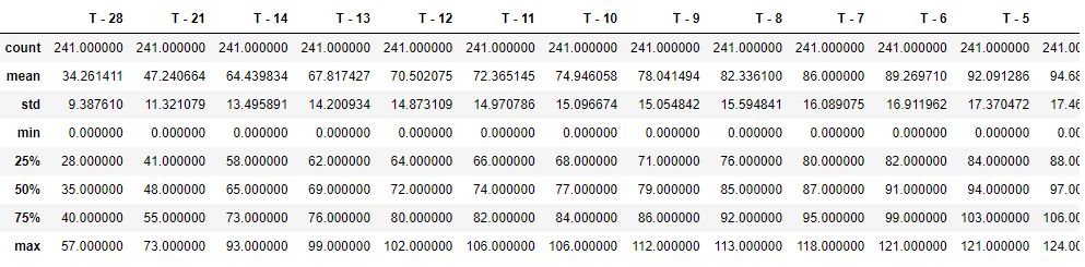
Let’s get the descriptive statistics info
df.describe()
Let’s calculate correlations
df.corr()
| T – 28 | T – 21 | T – 14 | T – 13 | T – 12 | T – 11 | T – 10 | T – 9 | T – 8 | T – 7 | T – 6 | T – 5 | T – 4 | T – 3 | T – 2 | T – 1 | Actual | |
|---|---|---|---|---|---|---|---|---|---|---|---|---|---|---|---|---|---|
| T – 28 | 1.000000 | 0.894700 | 0.766981 | 0.761258 | 0.764272 | 0.769680 | 0.744281 | 0.718607 | 0.697891 | 0.669865 | 0.669421 | 0.679711 | 0.685468 | 0.686128 | 0.655022 | 0.629432 | 0.608290 |
| T – 21 | 0.894700 | 1.000000 | 0.871427 | 0.862506 | 0.849120 | 0.839669 | 0.821875 | 0.807351 | 0.794639 | 0.769279 | 0.771311 | 0.766765 | 0.766230 | 0.763745 | 0.742956 | 0.718364 | 0.702459 |
| T – 14 | 0.766981 | 0.871427 | 1.000000 | 0.975593 | 0.940374 | 0.918844 | 0.913420 | 0.924774 | 0.919929 | 0.900452 | 0.890108 | 0.863536 | 0.846024 | 0.845696 | 0.848112 | 0.821478 | 0.800877 |
| T – 13 | 0.761258 | 0.862506 | 0.975593 | 1.000000 | 0.977337 | 0.955026 | 0.941554 | 0.940412 | 0.931122 | 0.914450 | 0.911955 | 0.895554 | 0.878267 | 0.870565 | 0.862705 | 0.835040 | 0.812730 |
| T – 12 | 0.764272 | 0.849120 | 0.940374 | 0.977337 | 1.000000 | 0.986618 | 0.962074 | 0.941533 | 0.922158 | 0.904064 | 0.912807 | 0.919413 | 0.910958 | 0.893899 | 0.876955 | 0.847387 | 0.818714 |
| T – 11 | 0.769680 | 0.839669 | 0.918844 | 0.955026 | 0.986618 | 1.000000 | 0.979289 | 0.947764 | 0.918142 | 0.896470 | 0.906488 | 0.920257 | 0.923938 | 0.908863 | 0.885674 | 0.851878 | 0.819855 |
| T – 10 | 0.744281 | 0.821875 | 0.913420 | 0.941554 | 0.962074 | 0.979289 | 1.000000 | 0.973322 | 0.935192 | 0.912204 | 0.918598 | 0.922247 | 0.927982 | 0.926197 | 0.907966 | 0.871200 | 0.842193 |
| T – 9 | 0.718607 | 0.807351 | 0.924774 | 0.940412 | 0.941533 | 0.947764 | 0.973322 | 1.000000 | 0.971532 | 0.955061 | 0.945678 | 0.933364 | 0.925826 | 0.924528 | 0.922874 | 0.895139 | 0.872890 |
| T – 8 | 0.697891 | 0.794639 | 0.919929 | 0.931122 | 0.922158 | 0.918142 | 0.935192 | 0.971532 | 1.000000 | 0.984829 | 0.969236 | 0.948335 | 0.930065 | 0.920350 | 0.927708 | 0.909233 | 0.887675 |
| T – 7 | 0.669865 | 0.769279 | 0.900452 | 0.914450 | 0.904064 | 0.896470 | 0.912204 | 0.955061 | 0.984829 | 1.000000 | 0.984542 | 0.960000 | 0.938392 | 0.925503 | 0.934284 | 0.918124 | 0.895779 |
| T – 6 | 0.669421 | 0.771311 | 0.890108 | 0.911955 | 0.912807 | 0.906488 | 0.918598 | 0.945678 | 0.969236 | 0.984542 | 1.000000 | 0.983981 | 0.963228 | 0.946564 | 0.950649 | 0.927954 | 0.898900 |
| T – 5 | 0.679711 | 0.766765 | 0.863536 | 0.895554 | 0.919413 | 0.920257 | 0.922247 | 0.933364 | 0.948335 | 0.960000 | 0.983981 | 1.000000 | 0.984911 | 0.964317 | 0.959692 | 0.937331 | 0.902827 |
| T – 4 | 0.685468 | 0.766230 | 0.846024 | 0.878267 | 0.910958 | 0.923938 | 0.927982 | 0.925826 | 0.930065 | 0.938392 | 0.963228 | 0.984911 | 1.000000 | 0.984158 | 0.968785 | 0.943132 | 0.906040 |
| T – 3 | 0.686128 | 0.763745 | 0.845696 | 0.870565 | 0.893899 | 0.908863 | 0.926197 | 0.924528 | 0.920350 | 0.925503 | 0.946564 | 0.964317 | 0.984158 | 1.000000 | 0.983117 | 0.950928 | 0.913242 |
| T – 2 | 0.655022 | 0.742956 | 0.848112 | 0.862705 | 0.876955 | 0.885674 | 0.907966 | 0.922874 | 0.927708 | 0.934284 | 0.950649 | 0.959692 | 0.968785 | 0.983117 | 1.000000 | 0.970063 | 0.936430 |
| T – 1 | 0.629432 | 0.718364 | 0.821478 | 0.835040 | 0.847387 | 0.851878 | 0.871200 | 0.895139 | 0.909233 | 0.918124 | 0.927954 | 0.937331 | 0.943132 | 0.950928 | 0.970063 | 1.000000 | 0.964727 |
| Actual | 0.608290 | 0.702459 | 0.800877 | 0.812730 | 0.818714 | 0.819855 | 0.842193 | 0.872890 | 0.887675 | 0.895779 | 0.898900 | 0.902827 | 0.906040 | 0.913242 | 0.936430 | 0.964727 | 1.000000 |
We can plot the correlation matrix as an image
f = plt.figure(figsize=(19, 15))
plt.matshow(df.corr(), fignum=f.number)
plt.xticks(range(df.select_dtypes([‘number’]).shape[1]), df.select_dtypes([‘number’]).columns, fontsize=14, rotation=45)
plt.yticks(range(df.select_dtypes([‘number’]).shape[1]), df.select_dtypes([‘number’]).columns, fontsize=14)
cb = plt.colorbar()
cb.ax.tick_params(labelsize=14)
plt.title(‘Correlation Matrix’, fontsize=16);
plt.savefig(‘corrmatrix.png’)

or a lower triangular matrix with annotations

We can see that the surgery volume correlation value decreases as the gap from the surgery day increases.
Let’s look at the mean and std of the Actual data grouped by DOW
df.groupby(‘DOW’)[‘Actual’].mean(), df.groupby(‘DOW’)[‘Actual’].std()
(DOW
 Fri    105.612245
 Mon    116.255319
 Thu    124.083333
 Tue    119.081633
 Wed    117.041667
 Name: Actual, dtype: float64,
 DOW
 Fri    26.357175
 Mon    18.456138
 Thu    10.379672
 Tue    10.864385
 Wed    11.240047
 Name: Actual, dtype: float64)
Let’s look at the mean and std of the T-1 data grouped by DOW
df.groupby(‘DOW’)[‘T – 1’].mean(), df.groupby(‘DOW’)[‘T – 1’].std()
(DOW
 Fri     97.428571
 Mon    110.787234
 Thu    117.583333
 Tue    114.020408
 Wed    110.416667
 Name: T - 1, dtype: float64,
 DOW
 Fri    25.922159
 Mon    18.863279
 Thu    10.394011
 Tue    10.296621
 Wed    11.100764
 Name: T - 1, dtype: float64)
Let’s calculate the number of surgeries per weekday
df[‘DOW’].value_counts()
Tue    49
Fri    49
Wed    48
Thu    48
Mon    47
Name: DOW, dtype: int64
Let’s create the barplot Actual-DOW
df2 = df[[‘DOW’, ‘Actual’]]
sns.color_palette(“flare”, as_cmap=True)
ax = sns.barplot(x=’DOW’,y=’Actual’, data=df)
ax.set(ylim=(80, 130))
plt.savefig(‘barplotactualdow.png’)

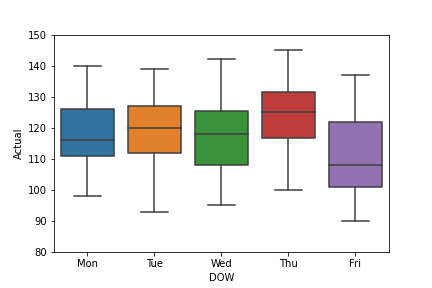
The corresponding boxplot is as follows
sns.color_palette(“flare”, as_cmap=True)
ax=sns.boxplot(x=’DOW’,y=’Actual’, data=df)
ax.set(ylim=(80, 150))
plt.savefig(‘boxplotactualdow.png’)
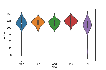
We can also look at the violine plot
sns.color_palette(“flare”, as_cmap=True)
ax=sns.violinplot(x=’DOW’,y=’Actual’, data=df)
plt.savefig(‘violineplotactualdow.png’)
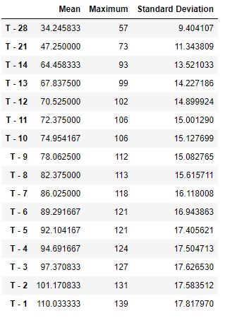
Let’s create the table new with 3 columns [‘Mean’, ‘Maximum’, ‘Standard Deviation’]
test=df.loc[1:242, ‘T – 28′:’T – 1’]
mean = test.mean()
maximum = test.max()
std = test.std()
a = pd.DataFrame(mean)
b = pd.DataFrame(maximum)
c = pd.DataFrame(std)
new = pd.concat([a,b,c], axis = 1)
new.columns = [‘Mean’, ‘Maximum’, ‘Standard Deviation’]
new
Let’s perform the OLS fitting while running the ANOVA H0-H1 test
import statsmodels.api as sm
from statsmodels.formula.api import ols
model = ols(‘Actual ~ DOW’, data=df).fit()
aov_table = sm.stats.anova_lm(model, typ=2)
aov_table
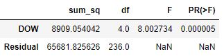
We reject the H0 hypothesis at the 99% confidence since p-value is less than 0.05.
Let’s perform multiple pairwise comparison of mean surgery volumes using the Tukey HSD test. The idea is to examine the difference between daily surgery volumes by taking various combinations of any two (randomly selected) weekdays
from statsmodels.stats.multicomp import pairwise_tukeyhsd
tukey = pairwise_tukeyhsd(endog=df[‘Actual’], groups=df[‘DOW’], alpha=0.05)
print(tukey)
 Multiple Comparison of Means - Tukey HSD, FWER=0.05
=====================================================
group1 group2 meandiff p-adj   lower    upper  reject
-----------------------------------------------------
   Fri    Mon  10.6431  0.017   1.2798 20.0063   True
   Fri    Thu  18.4711    0.0   9.1577 27.7844   True
   Fri    Tue  13.4694 0.0008   4.2042 22.7346   True
   Fri    Wed  11.4294 0.0077   2.1161 20.7428   True
   Mon    Thu    7.828 0.1529  -1.5829 17.2389  False
   Mon    Tue   2.8263 0.9212   -6.537 12.1896  False
   Mon    Wed   0.7863 0.9994  -8.6246 10.1972  False
   Thu    Tue  -5.0017 0.5789 -14.3151  4.3117  False
   Thu    Wed  -7.0417 0.2376 -16.4029  2.3196  False
   Tue    Wed    -2.04 0.9747 -11.3533  7.2734  False
-----------------------------------------------------
This test confirms significant differences between various combinations of daily surgery volumes by considering any two (randomly selected) weekdays.
We are ready to build and deploy our regression model(s).
Let’s prepare the data by excluding the ouliers (cf. boxplot and violineplot)
df1 = df.drop(columns = [‘SurgDate’, ‘DOW’])
from scipy import stats
df1 = df1[(np.abs(stats.zscore(df1)) < 3).all(axis=1)]
Let’s begin with the T-1, T-2, and T-3 variables x being related to the target variable y as follows
x = df[[‘T – 3’, ‘T – 2’, ‘T – 1’]]
y = df[[‘Actual’]]
First, let’s try sklearn linear_model
from sklearn import linear_model
import statsmodels.api as sm
regr = linear_model.LinearRegression()
regr.fit(x, y)
print(‘Intercept: \n’, regr.intercept_)
print(‘Coefficients: \n’, regr.coef_)
Intercept:
 [10.96140663]
Coefficients:
 [[-0.14256711  0.15693554  0.94016588]]
Second, we invoke OLS statsmodels
model = sm.OLS(y, x).fit()
predictions = model.predict(x)
print_model = model.summary()
print(print_model)
OLS Regression Results
=======================================================================================
Dep. Variable:                 Actual   R-squared (uncentered):                   0.998
Model:                            OLS   Adj. R-squared (uncentered):              0.998
Method:                 Least Squares   F-statistic:                          4.535e+04
Date:                Mon, 27 Jun 2022   Prob (F-statistic):                        0.00
Time:                        11:39:33   Log-Likelihood:                         -725.88
No. Observations:                 241   AIC:                                      1458.
Df Residuals:                     238   BIC:                                      1468.
Df Model:                           3
Covariance Type:            nonrobust
==============================================================================
                 coef    std err          t      P>|t|      [0.025      0.975]
------------------------------------------------------------------------------
T - 3         -0.1908      0.099     -1.926      0.055      -0.386       0.004
T - 2          0.1453      0.127      1.144      0.254      -0.105       0.395
T - 1          1.0908      0.069     15.891      0.000       0.956       1.226
==============================================================================
Omnibus:                        4.980   Durbin-Watson:                   1.916
Prob(Omnibus):                  0.083   Jarque-Bera (JB):                4.972
Skew:                           0.245   Prob(JB):                       0.0833
Kurtosis:                       3.506   Cond. No.                         89.7
==============================================================================

Notes:
[1] R² is computed without centering (uncentered) since the model does not contain a constant.
[2] Standard Errors assume that the covariance matrix of the errors is correctly specified.
We can also fit the simple linear regression model
from sklearn.linear_model import LinearRegression
regressorObject=LinearRegression()
regressorObject.fit(x,y)
Predict the number of surgeries:
predict = df1.loc[2:242, ‘T – 3′:’T – 1’]
y_pred_test_data=regressorObject.predict(predict)
Predicted = pd.DataFrame(y_pred_test_data, columns = [‘Predicted’])
result = pd.concat([df, Predicted], ignore_index=True, axis=1)
result.columns = [‘SurgDate’, ‘DOW’, ‘T – 28’, ‘T – 21’, ‘T – 14’, ‘T – 13’, ‘T – 12’, ‘T – 11′,’ T – 10′, ‘T – 9’,
‘T – 8’, ‘T – 7’, ‘T – 6’, ‘T – 5’, ‘T – 4’, ‘T – 3’, ‘T – 2’, ‘T – 1’, ‘Actual’, ‘Predicted’]
result[‘Predicted’] = round(result[‘Predicted’])
final = result.dropna()
final.tail(10)

Let’s calculate RMS
from sklearn.metrics import mean_squared_error
from math import sqrt
y_actual = final[‘Actual’]
y_predicted = final[‘Predicted’]
rms = sqrt(mean_squared_error(y_actual, y_predicted))
rms
20.653782302625718
Let’s calculate other performance metrics
y = final[‘Actual’]
yhat = final[‘Predicted’]
d = y – yhat
mse_f = np.mean(d2)
mae_f = np.mean(abs(d)) rmse_f = np.sqrt(mse_f) r2_f = 1-(sum(d2)/sum((y-np.mean(y))**2))
print(“Results by manual calculation:”)
print(“MAE:”,mae_f)
print(“MSE:”, mse_f)
print(“RMSE:”, rmse_f)
print(“R-Squared:”, r2_f)
Results by manual calculation:
MAE: 14.953191489361702
MSE: 426.5787234042553
RMSE: 20.653782302625718
R-Squared: -0.3528353839078937
Recall that the above model was applied to the three variables ‘T – 3′:’T – 1’.
Now let us consider 16 variables. We want to predict results for 3 days before the Surgery Date
x = df1[[‘T – 28’, ‘T – 21’, ‘T – 14’, ‘T – 13’, ‘T – 12’, ‘T – 11’, ‘T – 10’, ‘T – 9’, ‘T – 8’, ‘T – 7’,
‘T – 6’, ‘T – 5’, ‘T – 4’, ‘T – 3’, ‘T – 2’, ‘T – 1’]]
y = df1[[‘Actual’]]
by predicting results for 3 days before the Surgery Date.
Let’s re-apply our regression models
With sklearn linear_model
from sklearn import linear_model
import statsmodels.api as sm
regr = linear_model.LinearRegression()
regr.fit(x, y)
print(‘Intercept: \n’, regr.intercept_)
print(‘Coefficients: \n’, regr.coef_)
Intercept:
 [14.84638197]
Coefficients:
 [[-0.03590406  0.0856059  -0.10080439  0.07939623  0.08764874 -0.20750371
   0.03761113  0.10250478  0.00932406  0.12867575 -0.11420405 -0.03460241
   0.06443631 -0.15945052  0.12085577  0.87903786]]
With OLS statsmodels
model = sm.OLS(y, x).fit()
predictions = model.predict(x)
print_model = model.summary()
print(print_model)
OLS Regression Results
=======================================================================================
Dep. Variable:                 Actual   R-squared (uncentered):                   0.998
Model:                            OLS   Adj. R-squared (uncentered):              0.998
Method:                 Least Squares   F-statistic:                              8646.
Date:                Mon, 27 Jun 2022   Prob (F-statistic):                   4.06e-299
Time:                        11:58:15   Log-Likelihood:                         -705.05
No. Observations:                 237   AIC:                                      1442.
Df Residuals:                     221   BIC:                                      1498.
Df Model:                          16
Covariance Type:            nonrobust
==============================================================================
                 coef    std err          t      P>|t|      [0.025      0.975]
------------------------------------------------------------------------------
T - 28        -0.0402      0.079     -0.507      0.612      -0.196       0.116
T - 21         0.0955      0.084      1.142      0.254      -0.069       0.260
T - 14        -0.1061      0.126     -0.845      0.399      -0.354       0.141
T - 13         0.1548      0.189      0.821      0.413      -0.217       0.526
T - 12        -0.0594      0.214     -0.278      0.781      -0.480       0.362
T - 11        -0.0900      0.210     -0.429      0.669      -0.504       0.324
T - 10        -0.0144      0.168     -0.086      0.932      -0.345       0.316
T - 9          0.1131      0.150      0.756      0.451      -0.182       0.408
T - 8         -0.0078      0.152     -0.052      0.959      -0.307       0.291
T - 7          0.2021      0.178      1.133      0.259      -0.149       0.554
T - 6         -0.1933      0.193     -1.002      0.317      -0.573       0.187
T - 5         -0.0897      0.182     -0.492      0.623      -0.448       0.269
T - 4          0.1104      0.183      0.605      0.546      -0.249       0.470
T - 3         -0.1945      0.159     -1.227      0.221      -0.507       0.118
T - 2          0.1490      0.138      1.083      0.280      -0.122       0.420
T - 1          1.0405      0.072     14.501      0.000       0.899       1.182
==============================================================================
Omnibus:                        6.221   Durbin-Watson:                   1.995
Prob(Omnibus):                  0.045   Jarque-Bera (JB):                7.642
Skew:                           0.204   Prob(JB):                       0.0219
Kurtosis:                       3.779   Cond. No.                         314.
==============================================================================

Notes:
[1] R² is computed without centering (uncentered) since the model does not contain a constant.
[2] Standard Errors assume that the covariance matrix of the errors is correctly specified.
Fitting Simple Linear regression data model
from sklearn.linear_model import LinearRegression
regressorObject=LinearRegression()
regressorObject.fit(x,y)
Predicting the number of surgeries
predict = df1.loc[2:242, ‘T – 28′:’T – 1’]
y_pred_test_data=regressorObject.predict(predict)
Predicted = pd.DataFrame(y_pred_test_data, columns = [‘Predicted’])
result2 = pd.concat([df, Predicted], ignore_index=True, axis=1)
result2.columns = [‘SurgDate’, ‘DOW’, ‘T – 28’, ‘T – 21’, ‘T – 14’, ‘T – 13’, ‘T – 12’, ‘T – 11′,’ T – 10′, ‘T – 9’,
‘T – 8’, ‘T – 7’, ‘T – 6’, ‘T – 5’, ‘T – 4’, ‘T – 3’, ‘T – 2’, ‘T – 1’, ‘Actual’, ‘Predicted’]
result2[‘Predicted’] = round(result2[‘Predicted’])
final2 = result2.dropna()
round(result[‘Actual’].mean()), round(result2[‘Predicted’].mean())
(116, 118)
We can see that the Average Daily Error of surgeries is ~2 Surgeries.
Let’s check RMS
from sklearn.metrics import mean_squared_error
from math import sqrt
y_actual = final2[‘Actual’]
y_predicted = final2[‘Predicted’]
rms = sqrt(mean_squared_error(y_actual, y_predicted))
rms
20.367475114829315
Let’s calculate other performance metrics
y = final2[‘Actual’]
yhat = final2[‘Predicted’]
d = y – yhat
mse_f = np.mean(d2) mae_f = np.mean(abs(d)) rmse_f = np.sqrt(mse_f) r2_f = 1-(sum(d2)/sum((y-np.mean(y))**2))
print(“Results by manual calculation:”)
print(“MAE:”,mae_f)
print(“MSE:”, mse_f)
print(“RMSE:”, rmse_f)
print(“R-Squared:”, r2_f)
Results by manual calculation:
MAE: 14.697872340425532
MSE: 414.83404255319147
RMSE: 20.367475114829315
R-Squared: -0.3155887540215563
Predicting results for 7 days before the surgery date.
Let’s set x and y
x = df1[[‘T – 28’, ‘T – 21’, ‘T – 14’, ‘T – 13’, ‘T – 12’, ‘T – 11’, ‘T – 10’, ‘T – 9’, ‘T – 8’]]
y = df1[[‘Actual’]]
Fitting Simple Linear regression data model
from sklearn.linear_model import LinearRegression
regressorObject=LinearRegression()
regressorObject.fit(x,y)
Predicting the number of surgeries
predict = df1.loc[2:242, ‘T – 28′:’T – 8’]
y_pred_test_data=regressorObject.predict(predict)
Predicted = pd.DataFrame(y_pred_test_data, columns = [‘Predicted’])
result3 = pd.concat([df, Predicted], ignore_index=True, axis=1)
result3.columns = [‘SurgDate’, ‘DOW’, ‘T – 28’, ‘T – 21’, ‘T – 14’, ‘T – 13’, ‘T – 12’, ‘T – 11′,’ T – 10′, ‘T – 9’,
‘T – 8’, ‘T – 7’, ‘T – 6’, ‘T – 5’, ‘T – 4’, ‘T – 3’, ‘T – 2’, ‘T – 1’, ‘Actual’, ‘Predicted’]
result3[‘Predicted’] = round(result3[‘Predicted’])
final3 = result3.dropna()
round(result[‘Actual’].mean()), round(final3[‘Predicted’].mean())
(116, 118)
We see that the Average Daily Error is ~2 Surgeries.
Let’s check the performance
y = final3[‘Actual’]
yhat = final3[‘Predicted’]
d = y – yhat
mse_f = np.mean(d2) mae_f = np.mean(abs(d)) rmse_f = np.sqrt(mse_f) r2_f = 1-(sum(d2)/sum((y-np.mean(y))**2))
print(“Results by manual calculation:”)
print(“MAE:”,mae_f)
print(“MSE:”, mse_f)
print(“RMSE:”, rmse_f)
print(“R-Squared:”, r2_f)
Results by manual calculation:
MAE: 13.565957446808511
MSE: 375.6085106382979
RMSE: 19.380622039508893
R-Squared: -0.19119040826349143
Let’s plot actual versus predicted values
plt.figure(figsize=[15,8])
plt.grid(True)
plt.plot(result[‘Actual’],label=’Actual’)
plt.plot(result[‘Predicted’],label=’Predicted’)
plt.ylim(80, 150)
plt.legend(loc=2)
plt.savefig(‘predictedactualdata.png’)

And the % relative error is
plt.figure(figsize=[15,8])
plt.grid(True)
plt.plot(100*abs((result[‘Actual’]-result[‘Predicted’])/result[‘Actual’]))
plt.ylim([0, 40])
plt.savefig(‘predictrelerror.png’)

Summary
Our input data have 4 outliers (11/25/2011, 12/23/2011, 12/26/2011, and 12/30/2011).
Our data analysis shows that Fridays/Thursdays have the lowest/highest number of surgeris.
The surgery volume correlation value between DOW and the actual Surgery Date (SD) decreases as the gap between DOW and SD increases.
The ANOVE test rejects our null hypothesis H0 with 99% confidence.
Our results are statistically significant since p<<0.05.
We have performed multiple pairwise comparison (Tukey HSD) test to confirm the acceptance of our H1 hypothesis.
Predicting surgery volumes for 7 days before the Surgery Date yields the best result, as shown below:
| Metric | Base Model | 3 Days Forecast | 7 Days Forecast |
| MAE | 14.95 | 14.69 | 13.56 |
| MSE | 426.57 | 414.83 | 375.60 |
| RMSE | 20.65 | 20.36 | 19.38 |
| R2 | -0.35 | -0.31 | -0.19 |
This project supports earlier studies [1, 2] in that it underlines the importance of the implementation of automatic registration systems that integrate into the work processes in the OR to collect more and better data.
References
[1] Edelman et al, Front Med (Lausanne). 2017; 4: 85.
Published online 2017 Jun 19. doi: 10.3389/fmed.2017.00085
[2] Eun et al, Decision Sciences, 07 August 2020
[3] Rashi Desai, 2021, Vanderbilt University Medical Center: Effective Surgery Schedule. Github Repository.
[4] Cem ÖZÇELİK, 2022, DATA SCIENCE PROJECT: PREDICTING THE AMOUNT OF SURGERY, Published in MLearning.ai.


Leave a comment