
Diabetes is a chronic disease that continues to be a significant and global concern since it affects the entire population’s health. It is a metabolic disorder that leads to high blood sugar levels and many other problems such as stroke, kidney failure, and heart and nerve problems.
About one in seven U.S. adults has diabetes now, according to the Centers for Disease Control and Prevention. But by 2050, that rate could skyrocket to as many as one in three.
Health experts and other stakeholders are working to develop categorization models that will aid in the prediction of diabetes and the formulation of preventative initiatives.
The objective of this study is to build a Machine Learning (ML) classifier model based on medical diagnostic measurements. This is a classic supervised binary classification problem.
a. Python-3 & Jupyter (Anaconda IDE)
b. Sample Diabetes Dataset
c. ML Libraries
The diabetes-2 data set PIDD was originated from UCI Machine Learning Repository and can be downloaded from here.
The dataset consists of 768 rows (female patients) and the following 8 columns (features):
- Number of times pregnant
- Plasma glucose concentration a 2 hours in an oral glucose tolerance test
- Diastolic blood pressure (mm Hg)
- Triceps skin fold thickness (mm)
- 2-Hour serum insulin (mu U/ml)
- Body mass index (weight in kg/(height in m)^2)
- Diabetes pedigree function
- Age (years)
In addition to the above features, the last 9th column of the dataset indicates if the person has been diagnosed with diabetes (1) or not (0).
Step 1: Dataset Reading and Editing
Let’s import/install Python libraries
import numpy as np
import pandas as pd
import matplotlib.pyplot as plt
import seaborn as sns
sns.set()
!pip install mlxtend
!pip install missingno
from mlxtend.plotting import plot_decision_regions
import missingno as msno
from pandas.plotting import scatter_matrix
from sklearn.preprocessing import StandardScaler
from sklearn.model_selection import train_test_split
from sklearn.neighbors import KNeighborsClassifier
from sklearn.metrics import confusion_matrix
from sklearn import metrics
from sklearn.metrics import classification_report
import warnings
warnings.filterwarnings(‘ignore’)
%matplotlib inline
Let’s read the csv dataset using Pandas
diabetes_df = pd.read_csv(‘YOUR_PATH/diabetes.csv’)
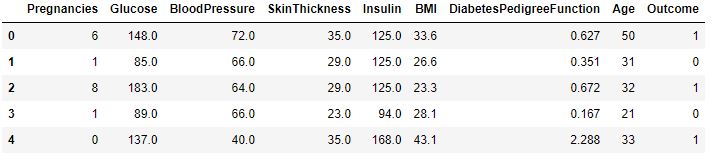
diabetes_df.head()

Step 2: Exploratory Data Analysis (EDA)
Let’s get the list of column names
diabetes_df.columns
Index(['Pregnancies', 'Glucose', 'BloodPressure', 'SkinThickness', 'Insulin',
       'BMI', 'DiabetesPedigreeFunction', 'Age', 'Outcome'],
      dtype='object')
diabetes_df.info()
<class 'pandas.core.frame.DataFrame'>
RangeIndex: 768 entries, 0 to 767
Data columns (total 9 columns):
 #   Column                    Non-Null Count  Dtype
---  ------                    --------------  -----
 0   Pregnancies               768 non-null    int64
 1   Glucose                   768 non-null    int64
 2   BloodPressure             768 non-null    int64
 3   SkinThickness             768 non-null    int64
 4   Insulin                   768 non-null    int64
 5   BMI                       768 non-null    float64
 6   DiabetesPedigreeFunction  768 non-null    float64
 7   Age                       768 non-null    int64
 8   Outcome                   768 non-null    int64
dtypes: float64(2), int64(7)
memory usage: 54.1 KB
diabetes_df.describe().T
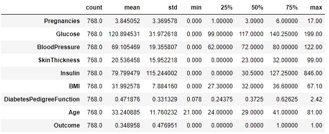
diabetes_df.isnull().sum()
Pregnancies                 0
Glucose                     0
BloodPressure               0
SkinThickness               0
Insulin                     0
BMI                         0
DiabetesPedigreeFunction    0
Age                         0
Outcome                     0
dtype: int64
diabetes_df_copy = diabetes_df.copy(deep = True)
diabetes_df_copy[[‘Glucose’,’BloodPressure’,’SkinThickness’,’Insulin’,’BMI’]] = diabetes_df_copy[[‘Glucose’,’BloodPressure’,’SkinThickness’,’Insulin’,’BMI’]].replace(0,np.NaN)
Showing the Count of NANs
print(diabetes_df_copy.isnull().sum())
Pregnancies                   0
Glucose                       5
BloodPressure                35
SkinThickness               227
Insulin                     374
BMI                          11
DiabetesPedigreeFunction      0
Age                           0
Outcome                       0
dtype: int64
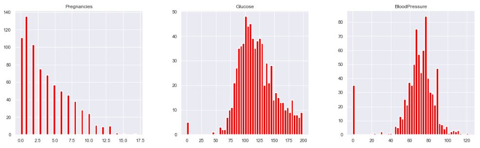
p = diabetes_df.hist(color = “red”, lw=2,bins=50,figsize = (20,20))


Let’s replace NaN with mean values:
diabetes_df_copy[‘Glucose’].fillna(diabetes_df_copy[‘Glucose’].mean(), inplace = True)
diabetes_df_copy[‘BloodPressure’].fillna(diabetes_df_copy[‘BloodPressure’].mean(), inplace = True)
diabetes_df_copy[‘SkinThickness’].fillna(diabetes_df_copy[‘SkinThickness’].median(), inplace = True)
diabetes_df_copy[‘Insulin’].fillna(diabetes_df_copy[‘Insulin’].median(), inplace = True)
diabetes_df_copy[‘BMI’].fillna(diabetes_df_copy[‘BMI’].median(), inplace = True)
Finally, let’s plot the outcome
color_wheel = {1: “#0392cf”, 2: “#7bc043”}
colors = diabetes_df[“Outcome”].map(lambda x: color_wheel.get(x + 1))
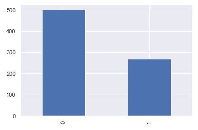
print(diabetes_df.Outcome.value_counts())
p=diabetes_df.Outcome.value_counts().plot(kind=”bar”)
0    500
1    268
Name: Outcome, dtype: int64
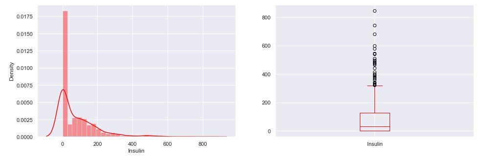
As an example, let’s plot aa selected distribution
plt.subplot(121), sns.distplot(diabetes_df[‘Insulin’],color = “red”)
plt.subplot(122), diabetes_df[‘Insulin’].plot.box(color = “red”,figsize=(16,5))
plt.show()
Step 3: Feature Engineering and Scaling
Let’s plot the heatmap symmetric 9×9 correlation matrix
plt.figure(figsize=(12,10))
Seaborn has an easy method to showcase heatmap
p = sns.heatmap(diabetes_df.corr(), annot=True,cmap =’RdYlGn’)

Let’s perform scaling the data
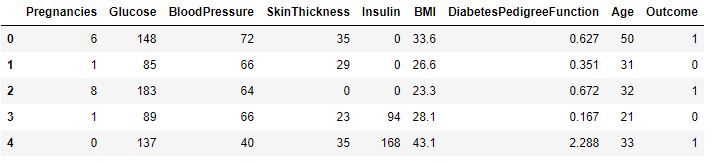
diabetes_df_copy.head()
sc_X = StandardScaler()
X = pd.DataFrame(sc_X.fit_transform(diabetes_df_copy.drop([“Outcome”],axis = 1),), columns=[‘Pregnancies’,
‘Glucose’, ‘BloodPressure’, ‘SkinThickness’, ‘Insulin’, ‘BMI’, ‘DiabetesPedigreeFunction’, ‘Age’])
X.head()

The last column remains the same
y = diabetes_df_copy.Outcome
y
0      1
1      0
2      1
3      0
4      1
      ..
763    0
764    0
765    0
766    1
767    0
Name: Outcome, Length: 768, dtype: int64
Step 4: Training and Testing the Model
X = diabetes_df.drop(‘Outcome’, axis=1)
y = diabetes_df[‘Outcome’]
Let’s split the data into the training and test datasets
from sklearn.model_selection import train_test_split
X_train, X_test, y_train, y_test = train_test_split(X,y, test_size=0.33,
random_state=7)
Random Forest Classifier
from sklearn.ensemble import RandomForestClassifier
rfc = RandomForestClassifier(n_estimators=200)
rfc.fit(X_train, y_train)
RandomForestClassifier(n_estimators=200)
rfc_train = rfc.predict(X_train)
from sklearn import metrics
print(“Accuracy_Score =”, format(metrics.accuracy_score(y_train, rfc_train)))
Accuracy_Score = 1.0
Let’s apply test predictions
from sklearn import metrics
predictions = rfc.predict(X_test)
print(“Accuracy_Score =”, format(metrics.accuracy_score(y_test, predictions)))
Accuracy_Score = 0.7834645669291339
Let’s produce the classification report
from sklearn.metrics import classification_report, confusion_matrix
print(confusion_matrix(y_test, predictions))
print(classification_report(y_test,predictions))
[[139  23]
 [ 32  60]]
              precision    recall  f1-score   support

           0       0.81      0.86      0.83       162
           1       0.72      0.65      0.69        92

    accuracy                           0.78       254
   macro avg       0.77      0.76      0.76       254
weighted avg       0.78      0.78      0.78       254
Decision Tree Classifier
from sklearn.tree import DecisionTreeClassifier
dtree = DecisionTreeClassifier()
dtree.fit(X_train, y_train)
DecisionTreeClassifier()
from sklearn import metrics
predictions = dtree.predict(X_test)
print(“Accuracy Score =”, format(metrics.accuracy_score(y_test,predictions)))
Accuracy Score = 0.7047244094488189
from sklearn.metrics import classification_report, confusion_matrix
print(confusion_matrix(y_test, predictions))
print(classification_report(y_test,predictions))
[[128  34]
 [ 39  53]]
              precision    recall  f1-score   support

           0       0.77      0.79      0.78       162
           1       0.61      0.58      0.59        92

    accuracy                           0.71       254
   macro avg       0.69      0.68      0.69       254
weighted avg       0.71      0.71      0.71       254
!pip install xgboost
from xgboost import XGBClassifier
xgb_model = XGBClassifier(gamma=0)
xgb_model.fit(X_train, y_train)
XGBClassifier(base_score=0.5, booster='gbtree', callbacks=None,
              colsample_bylevel=1, colsample_bynode=1, colsample_bytree=1,
              early_stopping_rounds=None, enable_categorical=False,
              eval_metric=None, gamma=0, gpu_id=-1, grow_policy='depthwise',
              importance_type=None, interaction_constraints='',
              learning_rate=0.300000012, max_bin=256, max_cat_to_onehot=4,
              max_delta_step=0, max_depth=6, max_leaves=0, min_child_weight=1,
              missing=nan, monotone_constraints='()', n_estimators=100,
              n_jobs=0, num_parallel_tree=1, predictor='auto', random_state=0,
              reg_alpha=0, reg_lambda=1, ...)
from sklearn import metrics
xgb_pred = xgb_model.predict(X_test)
print(“Accuracy Score =”, format(metrics.accuracy_score(y_test, xgb_pred)))
Accuracy Score = 0.7401574803149606
from sklearn.metrics import classification_report, confusion_matrix
print(confusion_matrix(y_test, xgb_pred))
print(classification_report(y_test,xgb_pred))
[[131  31]
 [ 35  57]]
              precision    recall  f1-score   support

           0       0.79      0.81      0.80       162
           1       0.65      0.62      0.63        92

    accuracy                           0.74       254
   macro avg       0.72      0.71      0.72       254
weighted avg       0.74      0.74      0.74       254
Support Vector Machine (SVM) Classifier
from sklearn.svm import SVC
svc_model = SVC()
svc_model.fit(X_train, y_train)
SVC()
svc_pred = svc_model.predict(X_test)
from sklearn import metrics
print(“Accuracy Score =”, format(metrics.accuracy_score(y_test, svc_pred)))
Accuracy Score = 0.7480314960629921
from sklearn.metrics import classification_report, confusion_matrix
print(confusion_matrix(y_test, svc_pred))
print(classification_report(y_test,svc_pred))
[[145  17]
 [ 47  45]]
              precision    recall  f1-score   support

           0       0.76      0.90      0.82       162
           1       0.73      0.49      0.58        92

    accuracy                           0.75       254
   macro avg       0.74      0.69      0.70       254
weighted avg       0.74      0.75      0.73       254
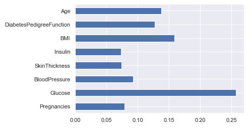
Feature Importance
rfc.feature_importances_
array([0.07883479, 0.25678968, 0.09288823, 0.07430253, 0.0730981 ,
       0.1584735 , 0.12750057, 0.13811259])
(pd.Series(rfc.feature_importances_, index=X.columns).plot(kind=’barh’))
<AxesSubplot:>
Saving Model – Random Forest
import pickle
#Firstly we will be using the dump() function to save the model using pickle
saved_model = pickle.dumps(rfc)
#Then we will be loading that saved model
rfc_from_pickle = pickle.loads(saved_model)
#Lastly, after loading that model we will use this to make predictions
rfc_from_pickle.predict(X_test)
array([0, 1, 1, 0, 0, 1, 0, 0, 1, 0, 1, 0, 1, 1, 0, 0, 0, 0, 0, 0, 0, 0,
       1, 1, 0, 0, 0, 0, 0, 0, 0, 0, 0, 1, 0, 0, 1, 0, 1, 0, 1, 1, 1, 0,
       0, 0, 1, 1, 0, 0, 0, 0, 0, 0, 1, 0, 0, 0, 0, 0, 0, 1, 0, 1, 1, 1,
       0, 1, 1, 1, 1, 1, 0, 0, 0, 0, 0, 0, 0, 0, 0, 0, 0, 0, 0, 0, 1, 0,
       1, 0, 1, 0, 1, 0, 0, 1, 1, 0, 0, 1, 0, 0, 0, 0, 0, 0, 0, 0, 0, 1,
       0, 1, 0, 0, 1, 0, 0, 0, 0, 1, 0, 0, 0, 0, 0, 1, 0, 1, 0, 0, 0, 1,
       0, 0, 0, 0, 0, 0, 0, 1, 0, 0, 1, 1, 0, 0, 0, 0, 1, 0, 0, 0, 0, 0,
       0, 0, 1, 0, 1, 0, 0, 0, 0, 0, 1, 0, 1, 0, 0, 1, 0, 1, 0, 0, 0, 0,
       1, 0, 1, 0, 1, 0, 0, 0, 0, 0, 0, 0, 0, 1, 1, 0, 1, 1, 0, 0, 1, 0,
       0, 0, 1, 0, 1, 1, 0, 0, 1, 0, 0, 0, 1, 1, 0, 0, 1, 0, 0, 1, 0, 0,
       0, 1, 1, 0, 1, 1, 0, 0, 1, 0, 0, 1, 0, 0, 0, 0, 0, 1, 1, 0, 1, 1,
       1, 0, 1, 0, 1, 0, 0, 0, 0, 1, 1, 1], dtype=int64)
diabetes_df.head()
rfc.predict([[0,137,40,35,168,43.1,2.228,33]]) #4th patient
array([1], dtype=int64)
rfc.predict([[10,101,76,48,180,32.9,0.171,63]]) # 763 th patient
array([0], dtype=int64)
plt.hist(y_test)
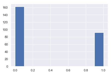
plt.hist(svc_pred)
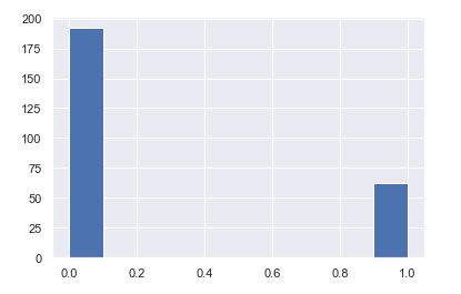
After using all these patient records, we are able to build a machine learning model (Random Forest – best one) to accurately predict whether or not the patients in the dataset have diabetes or not along with that we were able to draw some insights from the data via data analysis and visualization.
Remarks
- It is clearly visible that Glucose as a feature is the most important in this dataset.
- We look at the head and tail of the dataset so that we can take any random set of features from both the head and tail of the data to test that if our model is good enough to give the right prediction.
- The feature importance chart shows relative feature weights determined the during model building phase.
- We split the data into training and testing data using the train_test_split function with the parameter
test_size=0.33
- Distplot is helpful to see the distribution of the data while boxplot shows outliers in the specific feature/column.
- The dataset is imbalanced in that the number of patients who are diabetic is half of the patients who are non-diabetic.
- There are no null values in the input dataset.
INFOGRAPHIC


Leave a comment