Featured Foto by AtHul K Anand on Pexels
- The Kalman Filter (KF) is an optimal estimator with numerous applications in technology, especially in systems with Gaussian distributed noise. It has many uses, including applications in control, navigation, computer vision, and time series econometrics.
- It’s about extracting a signal from noisy data, a process commonly referred to as estimation. KF essentially involves removing noise, or alternatively, it can be viewed as estimating the underlying signal from data corrupted with noise.
- Several use-case examples illustrate how to use KF for tracking objects and focus on three important features: (1) prediction of object’s future location; (2) reduction of noise introduced by inaccurate detections; (3) facilitating the process of association of multiple objects to their tracks.
- In this posts, the sensitivity due to class of errors and data noise in the KF-based statistical modeling of object tracking will be discussed in great detail.
- The goal of this work is to get deep insights into the properties of (non)linear KF in order to make more informed decisions regarding the selection and tuning of these filters for different real-world applications.
- To address the noise/error sensitivity problem of KF, we will design our QC numerical experiments to test the mutual relations among the covariance matrices, their respective Kalman gain and the error covariance matrices.
- Scope: The KF equations will be numerically analyzed and designed based on noise/error components. Also, some values of measurement and variance constants will be simulated in Python and then the filtered result will be analyzed to obtain the optimized parameter value.
- Business Value: If the estimated KF states are used in a feedback controller, the accuracy and stability of the estimates becomes crucial for the safe and effective execution of the controller (e.g. aircraft control applications).
- Strategy: An Adaptive KF approach can be applied within the proposed framework in order to tune the measurement noise covariance and measurement mapping function of KF as the most important parameters affecting the filter’s performance.
Table of Contents
- Constant Voltage
- Alternating Current
- Linear Trend Path
- Non-Linear Trend Path
- Velocity Modeling
- Acceleration Modeling
- Circular Motion Robot
- 2D Location Tracking
- 3D Location Tracking
- Summary
- Explore More
- References
Constant Voltage
- Let’s begin with the basic linear KF algorithm and the corresponding demo that implement the example given in pages 11-15 of pages 11-15 of An Introduction to the Kalman Filter by Greg Welch and Gary Bishop, University of North Carolina at Chapel Hill, Department of Computer Science.
- Example: The UAV’s electronics need a constant voltage to function.
- Setting up working directory YOURPATH
import os
os.chdir('YOURPATH')    # Set working directory
os. getcwd()
- Running the KF code and plotting the result with different values of process variance Q and an estimate of measurement variance R
import numpy as np
import matplotlib.pyplot as plt

plt.rcParams['figure.figsize'] = (10, 8)

# intial parameters
n_iter = 100
sz = (n_iter,) # size of array


Q = 1e-6 # process variance, change to see effect

# allocate space for arrays
xhat=np.zeros(sz)      # a posteri estimate of x
P=np.zeros(sz)         # a posteri error estimate
xhatminus=np.zeros(sz) # a priori estimate of x
Pminus=np.zeros(sz)    # a priori error estimate
K=np.zeros(sz)         # gain or blending factor

R = 0.05**2 # estimate of measurement variance, change to see effect

# intial guesses
xhat[0] = 0.0
P[0] = 1.0

for k in range(1,n_iter):
    # time update
    xhatminus[k] = xhat[k-1]
    Pminus[k] = P[k-1]+Q

    # measurement update
    K[k] = Pminus[k]/( Pminus[k]+R )
    xhat[k] = xhatminus[k]+K[k]*(z[k]-xhatminus[k])
    P[k] = (1-K[k])*Pminus[k]

plt.figure()
plt.rcParams.update({'font.size': 14})
plt.plot(z,'k+',label='noisy measurements')
plt.plot(xhat,'b-',label='a posteriori estimate',lw=4)
plt.axhline(x,color='g',label='true value',lw=4)
plt.legend()
plt.title('Kalman Filter Q = 1e-5 R = 0.05**2', fontweight='bold')
plt.xlabel('Iteration')
plt.ylabel('Voltage')

plt.figure()
valid_iter = range(1,n_iter) # Pminus not valid at step 0
plt.plot(valid_iter,Pminus[valid_iter],label='a priori error estimate',lw=4)
plt.title('Estimated $\it{\mathbf{a \ priori}}$ error vs. iteration step', fontweight='bold')
plt.xlabel('Iteration')
plt.ylabel('$(Voltage)^2$')
plt.setp(plt.gca(),'ylim',[0,.01])
plt.show()

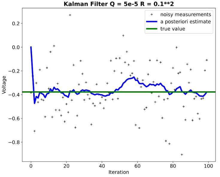
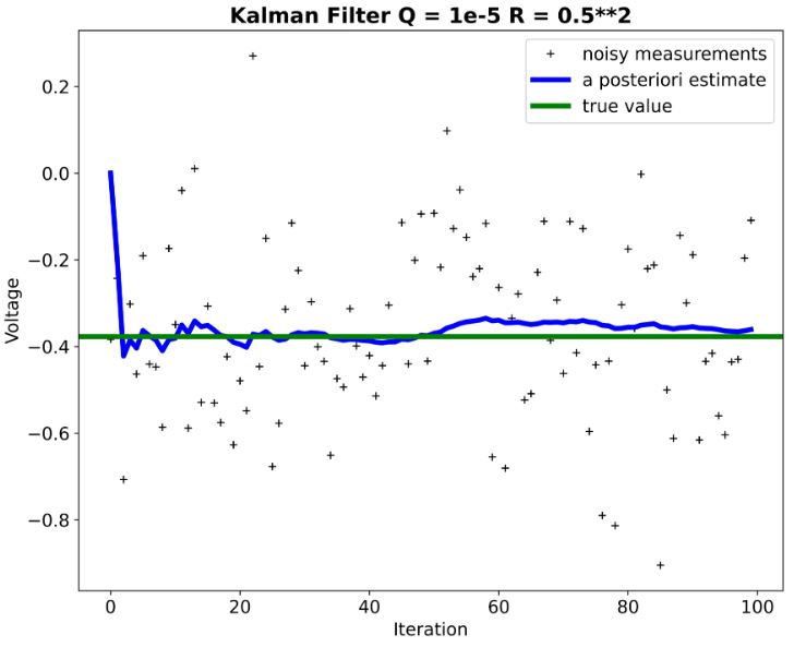
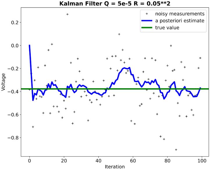
- We can see that KF performance is not extremely sensitive to deviations in the assumed process and measurement models.
- Remark: Negative voltage (see above plots) just means it’s negative relative to a reference point (usually ground). If you took a 1v battery and connected it’s positive terminal to ground, while leaving the negative terminal open, and then measured between it’s negative terminal and ground you would measure -1V.
Alternating Current
- The sinusoidal waveform (sine wave) is the fundamental
alternating current (AC) and alternating voltage waveform. - In this section, KF is tested with a noisy sine wave simulated by mixing a Gaussian white noise to a sine wave.
- Let’s implement the following KF algorithm
import numpy as np
import matplotlib.pyplot as plt
import math

Estimation_error = 0 # dynamic and looped
Measurement_variance = 100 #static, how confident you are in your sensors (in n*Var)
Process_noise_variance = 3 #Static, how confident you are in your model (in n*Var)

Model_error = 1/80 # this is how much our model guesses wrong, inject some constant to make it drift
#you shouldn't be able to change the model error in real life as it is limited by how rubbish your model is

def Kalman_gain(Eest, Emea):
    return Eest / (Eest + Emea)

def state_estimator(current, step_num):
    return current + time_step*np.cos(x_values[step_num]) + Model_error # introduce some consistent error to simulate integration error of a model

def corrected_estimate(prev_state_estimate, measurement, k):
    return prev_state_estimate + k*(measurement - prev_state_estimate)

def update_estimation_error(prev_estimation_error, k):
    return (1 - k) * prev_estimation_error + Proccess_noise_variance
# Generate data using a loop
num_steps = 100
x_values = np.linspace(0, 2 * np.pi, num_steps)
time_step = 2 * np.pi/num_steps

true_sine_wave = np.zeros(num_steps)
noisy_sine_wave = np.zeros(num_steps)
state_prediction = np.zeros(num_steps)
corrected_state = np.zeros(num_steps)
for i in range(num_steps):
    true_sine_wave[i] = np.sin(x_values[i])
    noisy_sine_wave[i] = true_sine_wave[i] + np.random.normal(0, 0.2)

    K = Kalman_gain(Estimation_error, Measurement_variance)
    # State prediction that is not corrected, will go into the cosmos
    state_prediction[i] = state_estimator(state_prediction[i-1], i)

    #state prediction correced by the noisy current signal
    corrected_state[i] = corrected_estimate(state_estimator(corrected_state[i-1], i), noisy_sine_wave[i], K)

    #lastly lets update the estimation error
    Estimation_error = update_estimation_error(Estimation_error, K)

# Plot the sine wave
plt.plot(x_values, true_sine_wave, label='True Sine Wave', color='blue')

# Plot the noisy sine wave
plt.plot(x_values, noisy_sine_wave, label='Noisy Sine Wave', color='red')

# Plot the state prediction
plt.plot(x_values, state_prediction, label='State Prediction (Raw)', color='green', linestyle='dashed')

plt.plot(x_values, corrected_state, label='State Prediction after Kalman (Corrected)', color='black')

# Add labels and title
plt.xlabel('X-axis')
plt.ylabel('Y-axis')
plt.title('True Sine Wave, Noisy Measurement, and State Prediction')

plt.rcParams['figure.dpi'] = 800
# Add a legend
plt.legend()

# Show the plot
plt.show()


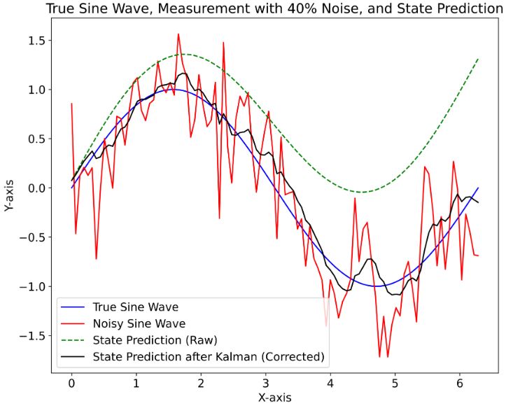
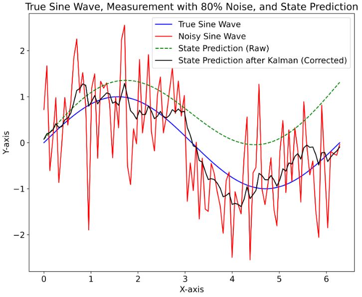
- This example explores one of the simplest wave motion models: a sine wave with constant amplitude and frequency.
- It confirms that the KF technique is suitable for noisy measurements with relatively low signal/noise ratios.
Linear Trend Path
- Let’s look at the relatively realistic KF approach to track the linear trajectory in the presence of noise.
"""
FilterPy library.
http://github.com/rlabbe/filterpy

Documentation at:
https://filterpy.readthedocs.org

Supporting book at:
https://github.com/rlabbe/Kalman-and-Bayesian-Filters-in-Python
"""

import numpy.random as random
import numpy as np
import matplotlib.pyplot as plt
from scipy.linalg import inv
from filterpy.kalman import KalmanFilter, InformationFilter

def test_1d():
    f = KalmanFilter (dim_x=2, dim_z=1)
    inf = InformationFilter (dim_x=2, dim_z=1)

    f.x = np.array([[2.],
                    [0.]])       # initial state (location and velocity)

    inf.x = f.x.copy()
    f.F = (np.array([[1.,1.],
                     [0.,1.]]))    # state transition matrix

    inf.F = f.F.copy()
    f.H = np.array([[1.,0.]])      # Measurement function
    inf.H = np.array([[1.,0.]])    # Measurement function
    f.R = 10.                       # state uncertainty
    inf.R_inv = 1./10               # state uncertainty
    f.Q = 0.000001                   # process uncertainty
    inf.Q = 0.000001

    m = []
    r = []
    r2 = []


    zs = []
    for t in range (100):
        # create measurement = t plus white noise
        z = t + random.randn()*10
        zs.append(z)

        # perform kalman filtering
        f.update(z)
        f.predict()

        inf.update(z)
        inf.predict()

        # save data
        r.append (f.x[0,0])
        r2.append (inf.x[0,0])
        m.append(z)

    if DO_PLOT:
        plt.plot(m,label='Measured')
        plt.plot(r)
        plt.plot(r2,label='Estimated',lw=4)
        plt.plot(m,m,label='True')
        plt.xlabel('X')
        plt.ylabel('Y')
        plt.xlim((-20, 120))
        plt.ylim((-20, 120))
        plt.legend()
        plt.title('Filterpy Kalman Filter: Noise=10% Q=1e-6 R=10')
        plt.grid()

if __name__ == "__main__":
    DO_PLOT = True
    test_1d()
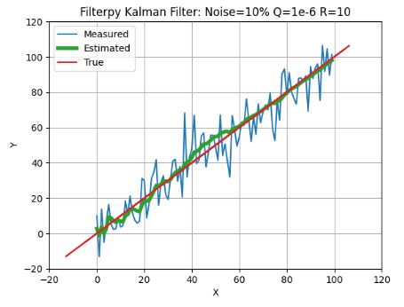


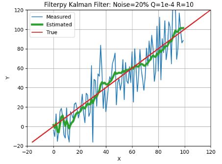
- This example shows that the FilterPy KF provides expected robustness against state/process uncertainty and the measurement (white) noise without sacrificing linear goodness-of-fit in the least squares sense.
Non-Linear Trend Path
- In fact, linearization along trajectories enables us to use KF concepts of linear time-varying systems for nonlinear systems.
- The position vs. time graphs for the two types of motion – constant velocity and changing velocity (acceleration) – are depicted as follows.
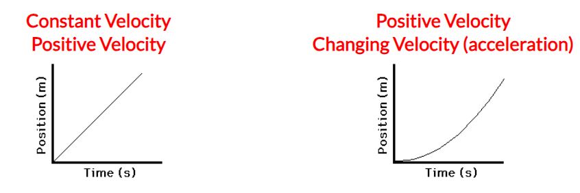
- Let’s look at the slope of the line on a position-time (p-t) graph. It is often said, “As the slope goes, so goes the velocity.” If the velocity is constant, then the slope is constant (i.e., a straight line). If the velocity is changing, then the slope is changing (i.e., a curved line). If the velocity is positive, then the slope is positive (i.e., moving upwards and to the right).
- The simple KF algorithm (and the Python code) that simulates a non-linear p-t curve is as follows:
class KalmanFilter(object):
    def __init__(self, dt, u, std_acc, std_meas):
        self.dt = dt
        self.u = u
        self.std_acc = std_acc
        self.A = np.matrix([[1, self.dt],
                            [0, 1]])
        self.B = np.matrix([[(self.dt**2)/2], [self.dt]])
        self.H = np.matrix([[1,0]])
        self.Q = np.matrix([[(self.dt**4)/4, (self.dt**3)/2],
                            [(self.dt**3)/2, self.dt**2]]) * self.std_acc**2
        self.R = std_meas**2
        self.P = np.eye(self.A.shape[1])
        self.x = np.matrix([[0],[0]])
    def predict(self):
        # Ref :Eq.(9) and Eq.(10)
        # Update time state
        self.x = np.dot(self.A, self.x) + np.dot(self.B, self.u)
        # Calculate error covariance
        # P= A*P*A' + Q
        self.P = np.dot(np.dot(self.A, self.P), self.A.T) + self.Q
        return self.x
    def update(self, z):
        # Ref :Eq.(11) , Eq.(11) and Eq.(13)
        # S = H*P*H'+R
        S = np.dot(self.H, np.dot(self.P, self.H.T)) + self.R
        # Calculate the Kalman Gain
        # K = P * H'* inv(H*P*H'+R)
        K = np.dot(np.dot(self.P, self.H.T), np.linalg.inv(S))  # Eq.(11)
        self.x = np.round(self.x + np.dot(K, (z - np.dot(self.H, self.x))))  # Eq.(12)
        I = np.eye(self.H.shape[1])
        self.P = (I - (K * self.H)) * self.P  # Eq.(13)
def main():
    dt = 0.1
    t = np.arange(0, 100, dt)
    # Define a model track
    real_track = 0.1*((t**2) - t)
    u= 4
    std_acc = 0.55     # we assume that the standard deviation of the acceleration is 0.25 (m/s^2)
    std_meas = 4.2    # and standard deviation of the measurement is 1.2 (m)
    # create KalmanFilter object
    kf = KalmanFilter(dt, u, std_acc, std_meas)
    predictions = []
    measurements = []
    for x in real_track:
        # Mesurement
        z = kf.H * x + np.random.normal(0, 100)
        measurements.append(z.item(0))
        predictions.append(kf.predict()[0])
        kf.update(z.item(0))
    fig = plt.figure(figsize=(15,6))
    fig.suptitle('Kalman Filter std_acc = 0.55 std_meas = 4.2 100 m Error std', fontsize=20)
    plt.plot(t, measurements, label='Measurements', color='b',linewidth=1)
    plt.plot(t, np.array(real_track), label='Real Track', color='y', linewidth=4)
    plt.plot(t, np.squeeze(predictions), label='Kalman Filter Prediction', color='r', linewidth=2)
    plt.xlabel('Time (s)', fontsize=20)
    plt.ylabel('Position (m)', fontsize=20)
    plt.legend()
    plt.grid()
    plt.show()
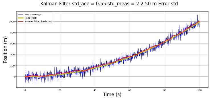
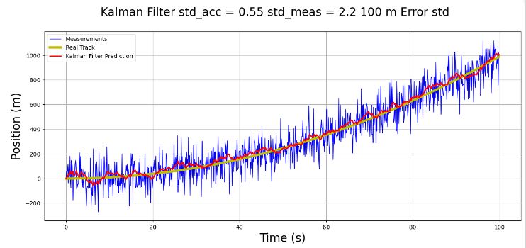


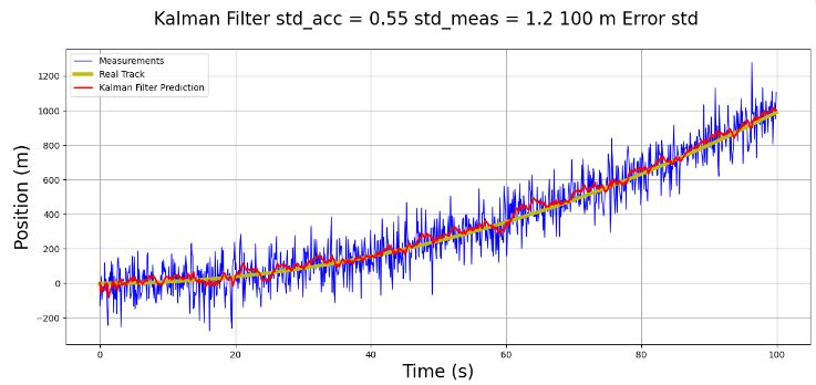
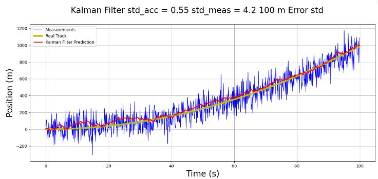
- This 1D p-t example serves as a prerequisite for testing 2D object tracking. It illustrates the concept of robust KF for discrete-time nonlinear systems with parameter uncertainties.
Velocity Modeling
- This example proposes a joint position and velocity estimation scheme for moving objects using KF.
- Business value: KF can estimate the position and velocity of a ground vehicle based on noisy position measurements such as GPS sensor measurements. The KF model can have time-varying noise characteristics.
- We have tried to use KF to estimate the position. The input in the system is the velocity and this is also what we measure. In practice, the velocity is often not stable, the system movement is like a cosine in general. One way would be to drop the velocities as inputs and put them in your KF state. This way, your state is both the position and velocity and your filter uses as observation both the measured speed of your vehicle and a noisy estimate of your position.
- Let’s implement the KF algorithm that yields estimates of the location and speed plus uncertainties:
#https://github.com/Vefot/Kalman-Filter/tree/master/python_kf
import numpy as np

# offsets of each variable in the state vector
iX = 0
iV = 1
NUMVARS = iV + 1


class KF:
    """
    One dimensional Kalman filter

    Instantiates with the following properties:

    initial_x: initial location
    initial_v: initial velocity
    accel_variance: variance in acceleration
    """

    def __init__(
        self, initial_x: float, initial_v: float, accel_variance: float
    ) -> None:
        # mean of state gaussian random variable
        self._x = np.zeros(NUMVARS)
        self._x[iX] = initial_x
        self._x[iV] = initial_v

        self._accel_variance = accel_variance

        # covariance matrix - represents uncertainty in the state
        self._P = np.eye(NUMVARS)  # eye returns a 2x2 identity matrix

    def predict(self, dt: float) -> None:
        """
        Predicts the state vector forward in time by dt (delta time) seconds
        """
        # x = F * x
        # p = F * p * F^T  * a

        # state transition matrix
        F = np.eye(NUMVARS)
        F[iX, iV] = dt

        # calculate the new state by multiplying state transition matrix with current x
        new_x = F.dot(self._x)

        # G - 2x1 matrix representing the control input (models affect of acceleration on position and velocity)
        # acceleration is assumed to be a random variable with a variance of accel_variance
        G = np.zeros((2, 1))
        G[iX] = 0.5 * dt**2
        G[iV] = dt
        # update covariance matrix (representing uncertainty in the state)
        new_P = F.dot(self._P).dot(F.T) + G.dot(G.T) * self._accel_variance

        self._P = new_P
        self._x = new_x

    def update(self, measurement_value: float, measurement_variance: float):
        # y = z - H x
        # S = H P Ht + R
        # K = P Ht S^-1
        # x = x + K y
        # P = (I - K H) * P

        H = np.zeros((1, NUMVARS))
        H[0, iX] = 1

        z = np.array([measurement_value])
        R = np.array([measurement_variance])

        y = z - H.dot(self._x)
        S = H.dot(self._P).dot(H.T) + R

        K = self._P.dot(H.T).dot(np.linalg.inv(S))

        new_x = self._x + K.dot(y)
        new_p = (np.eye(2) - K.dot(H)).dot(self._P)

        self._P = new_p
        self._x = new_x

    @property
    def covariance(self) -> np.array:
        """The covariance of the current state vector"""
        return self._P

    @property
    def mean(self) -> np.array:
        """The mean of the current state vector"""
        return self._x

    @property
    def pos(self) -> float:
        """The current position"""
        return self._x[iX]

    @property
    def vel(self) -> float:
        """The current velocity"""
        return self._x[iV]
from unittest import TestCase
import numpy as np
#from kf import KF


class TestKF(TestCase):
    def test_can_construct_with_x_and_v(self):
        """
        Tests that the KF class can be constructed with initial x and v
        and that the state vector is initialized with the correct values (x and v)
        """
        x = 0.2
        v = 2.3
        kf = KF(initial_x=x, initial_v=v, accel_variance=1.2)

        # test that the first element of the state vector is the initial x
        self.assertAlmostEqual(kf.pos, x)

        # test that the second element of the state vector is the initial v
        self.assertAlmostEqual(kf.vel, v)

    def test_after_calling_predict_x_and_p_are_right_shape(self):
        x = 0.2
        v = 2.3
        kf = KF(initial_x=x, initial_v=v, accel_variance=1.2)
        kf.predict(dt=0.1)

        # the covariance matrix should be 2x2
        self.assertEqual(kf.covariance.shape, (2, 2))

        # the state vector should be 2x1
        self.assertEqual(kf.mean.shape, (2,))

    def test_calling_predict_increases_state_uncertainty(self):
        """
        Uncertainty in the state should increase with time,
        so P should be larger after calling predict
        """
        x = 0.2
        v = 2.3
        kf = KF(initial_x=x, initial_v=v, accel_variance=1.2)

        for i in range(10):
            # det is the determinant of the covariance matrix (a measure of uncertainty in the state)
            det_before = np.linalg.det(kf.covariance)
            kf.predict(dt=0.1)
            det_after = np.linalg.det(kf.covariance)

            self.assertGreater(det_after, det_before)
            print(det_before, det_after)

    def test_calling_update_decreases_state_uncertainty(self):
        """
        Calling update should decrease uncertainty in the state
        because we are getting new information about the state
        from e.g. a sensor measurement
        """
        x = 0.2
        v = 2.3

        kf = KF(initial_x=x, initial_v=v, accel_variance=1.2)

        det_before = np.linalg.det(kf.covariance)
        kf.update(measurement_value=0.1, measurement_variance=0.01)
        det_after = np.linalg.det(kf.covariance)

        self.assertLess(det_after, det_before)
import numpy as np
import matplotlib.pyplot as plt
#from kf import KF

plt.ion()
plt.figure()

real_x = 0.0
measurement_variance = 1.5**2  # simulate noise in the measurement
real_v = 0.5

kf = KF(initial_x=0.0, initial_v=1.0, accel_variance=1.5)

DT = 0.1
NUM_STEPS = 1000
MEASUREMENT_EVERY_STEPS = 20


mus = []  # mean of the state
covs = []  # covariance
real_xs = []
real_vs = []

for step in range(NUM_STEPS):
    # change the speed after step 500..
    if step > 500:
        real_v *= 0.9

    covs.append(kf.covariance)
    mus.append(kf.mean)

    # update the position - simulate in this manner:
    real_x = real_x + DT * real_v

    kf.predict(dt=DT)

    # when we get a sensor reading, update the kalman filter
    # instead of giving the kf the real x we give it a slightly
    # noisy version
    if step != 0 and step % MEASUREMENT_EVERY_STEPS == 0:
        kf.update(
            measurement_value=real_x
            + np.random.randn() * np.sqrt(measurement_variance),
            measurement_variance=measurement_variance,
        )

    real_xs.append(real_x)
    real_vs.append(real_v)


plt.subplot(2, 1, 1)
plt.title("Kalman Filter meas_var = 1.5**2 accel_var=1.5")
plt.ylabel("Position")
# plot the mean of the state
plt.plot([mu[0] for mu in mus], "r",label='Kalman')
plt.plot(real_xs, "b",label='Real')
plt.legend()

# plot the uncertainty in the state - see a cone of uncertainty widening over time
plt.plot([mu[0] - 2 * np.sqrt(covs[0, 0]) for mu, covs in zip(mus, covs)], "r--")
plt.plot([mu[0] + 2 * np.sqrt(covs[0, 0]) for mu, covs in zip(mus, covs)], "r--")

plt.subplot(2, 1, 2)
plt.ylabel("Velocity")
plt.plot([mu[1] for mu in mus], "r",label='Kalman')
plt.plot(real_vs, "b",label='Real')
plt.xlabel("Time")

plt.plot([mu[1] - 2 * np.sqrt(covs[1, 1]) for mu, covs in zip(mus, covs)], "r--")
plt.plot([mu[1] + 2 * np.sqrt(covs[1, 1]) for mu, covs in zip(mus, covs)], "r--")

plt.legend()

plt.show()
plt.ginput(1)

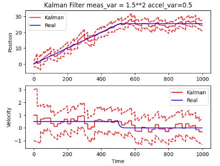

- This algorithm implements a method to obtain good synchronous and instantaneous estimates in position and velocity; using a position measurement only.
- Results show that the KF method allows for an increased accuracy and robustness of estimates with respect to the input measurement and acceleration variances. Since the method requires the measurement position only, it eliminates the need for more sensors for velocity.
Acceleration Modeling
- The KF is a commonly used tool to eliminate measurement noise occurring in the data most often taken from various sensors. The most common application is data filtration from accelerometers and gyroscopes, which are found, among others in smartphones and other modern devices.
- Let’s run the code that computes the acceleration using the Augmented Kalman Filter (AKF) and the Sequential Bayesian estimation of state.
#https://github.com/ingvft/Kalman_Filter/blob/master/main_full.py
# -*- coding: utf-8 -*-
"""
Created on Fri Nov 12 20:41:36 2021

@author: Victor Flores Terrazas at
        The Hong Kong University of Science and Technology

        Python implementation of original Matlab code from:
        * Sedehi, Omid, et al. "Sequential Bayesian estimation of
          state and input in dynamical systems using output-only measurements."
          Mechanical Systems and Signal Processing 131 (2019): 659-688.

        Implementation of Augmented Kalman Filter originally from Matlab code
        created by O. Sedehi, based on:
        * Lourens, E., et al. "An augmented Kalman filter for force
          identification in structural dynamics."
          Mechanical Systems and Signal Processing 27 (2012): 446-460.
"""

import numpy as np
import scipy.linalg as sc
import matplotlib.pyplot as plt

# ---------- Structural Model ---------------------------

M = np.identity(8)

C = np.array([[2, -1, 0, 0, 0, 0, 0, 0],
             [-1, 2, -1, 0, 0, 0, 0, 0],
             [0, -1, 2, -1, 0, 0, 0, 0],
             [0, 0, -1, 2, -1, 0, 0, 0],
             [0, 0, 0, -1, 2, -1, 0, 0],
             [0, 0, 0, 0, -1, 2, -1, 0],
             [0, 0, 0, 0, 0, -1, 2, -1],
             [0, 0, 0, 0, 0, 0, -1, 1]])

K = np.array([[2000, -1000, 0, 0, 0, 0, 0, 0],
              [-1000, 2000, -1000, 0, 0, 0, 0, 0],
              [0, -1000, 2000, -1000, 0, 0, 0, 0],
              [0, 0, -1000, 2000, -1000, 0, 0, 0],
              [0, 0, 0, -1000, 2000, -1000, 0, 0],
              [0, 0, 0, 0, -1000, 2000, -1000, 0],
              [0, 0, 0, 0, 0, -1000, 2000, -1000],
              [0, 0, 0, 0, 0, 0, -1000, 1000]])


# Define the number of DOFs of the model
ndof = np.shape(M)[1]

# Define the selection matrix for the input
nf = 1
Sp = np.zeros((ndof,nf))
Sp[0][0] = 1

# Define the continuous-time system matrices [Ac] and [Bc]

Z = np.zeros((ndof,ndof))
I = np.identity(ndof)
Ac = np.vstack((np.hstack((Z, I)),
               (np.hstack((-np.linalg.solve(M,K), -np.linalg.solve(M,C))))))
Bc = np.vstack((Z,np.linalg.solve(I.T,M.T))) @ Sp

# Define the discrete-time system matrices [A] and [B]

dt = 0.001
A = sc.expm(Ac * dt)
B = (A - np.identity(2*ndof)) @ np.linalg.inv(Ac) @ Bc

# ---------- Input ---------------------------

np.random.seed(1)

T = 50
Ndata = T/dt + 1
t = np.linspace(0, T, num=int(Ndata))
input_mu , input_std = 0 , 5
p_real = np.random.normal(input_mu, input_std, size=(int(Ndata),int(nf)))

# ---------- Structural Responses ---------------------------

Ge = np.vstack((np.hstack((I,Z)),
               (np.hstack((Z, I))),
               (np.hstack((-np.linalg.solve(M,K), -np.linalg.solve(M,C))))))
Je = np.vstack((Z,Z,np.linalg.solve(I.T,M.T))) @ Sp

# Pre-allocate matrices
x_real = np.zeros((2*ndof,int(Ndata)))
y_real = np.zeros((3*ndof,int(Ndata)))

# Initialize
x_real[:,0] = np.zeros((1,2*ndof))
y_real[:,0] = Ge @ x_real[:,0] + Je @ p_real[0,:]

for i in range(int(Ndata)-1):
    x_real[:,i+1] = A @ x_real[:,i] + B @ p_real[i,:]
    y_real[:,i+1] = Ge @ x_real[:,i] + Je @ p_real[i,:]


# ---------- Measurements ---------------------------
# np.random.seed(12)

na = 2
nv = 0
nd = 0
Sa = np.zeros((na,ndof))
Sa[0][0] = 1
Sa[1][3] = 1
G = Sa @ np.hstack([-np.linalg.solve(M,K), -np.linalg.solve(M,C)])
J = Sa @ np.linalg.solve(I.T,M.T) @ Sp

ry = np.var(y_real[19,:], axis = 0) * 0.01**2

nm = na + nv + nd

R = np.identity(nm) * ry

y_meas = np.zeros((int(nm),int(Ndata)))
meas_noise = np.random.normal(0,np.sqrt(ry),(int(nm),int(Ndata)))

for i in range(int(Ndata)-1):
    y_meas[:,i] = G @ x_real[:,i] + J @ p_real[i,:] + meas_noise[:,i]


# --------- Bayesian JISE -----------------

nu = 0
kappa = 1

Qx_bay = np.identity(int(2*ndof))*10**-3

x_bay = np.zeros((int(2*ndof),int(Ndata)))
p_bay = np.zeros((int(nf),int(Ndata)))
Px_bay = np.zeros((int(2*ndof),int(2*ndof),int(Ndata)))
Pp_bay = np.zeros((int(nf),int(nf),int(Ndata)))
Pxp_bay = np.zeros((int(2*ndof),int(nf),int(Ndata)))

Px_bay[:,:,0] = np.identity(Px_bay.shape[0])*Qx_bay
Pp_bay[:,:,0] = np.identity(Pp_bay.shape[0])*10**-3

mp = np.zeros((int(nf),int(Ndata)))
mpp = np.zeros((int(nf),int(Ndata)))
mx = np.zeros((int(2*ndof),int(Ndata)))
m = np.zeros((int(nm),int(Ndata)))

for i in range(int(Ndata)-1):
    # Time update for input and state
    Pp_bay[:,:,i+1] = Pp_bay[:,:,i]
    x_bay[:,i+1] = A @ x_bay[:,i]
    Px_bay[:,:,i+1] = ((A @ Px_bay[:,:,i] @ A.T) +
                       (B @ Pp_bay[:,:,i] @ B.T) +
                       (A @ Pxp_bay[:,:,i] @ B.T) +
                       (B @ Pxp_bay[:,:,i].T @ A.T) +
                       Qx_bay)

    # Kalman Gain matirx for input estimation
    Kp = Pp_bay[:,:,i+1] @ J.T @ (np.linalg.inv(J @ Pp_bay[:,:,i+1] @ J.T + R))

    # Measurement update for input
    p_bay[:,i+1] = Kp @ (y_meas[:,i+1] - G @ x_bay[:,i+1])
    Pp_bay[:,:,i+1] = (Pp_bay[:,:,i+1] +
                       Kp @ G @ Px_bay[:,:,i+1] @ G.T @ Kp.T -
                       Kp @ J @ Pp_bay[:,:,i+1])

    # Updating the state based on the new input
    x_bay[:,i+1] = A @ x_bay[:,i] + B @ p_bay[:,i]
    Px_bay[:,:,i+1] = ((A @ Px_bay[:,:,i] @ A.T) +
                       (B @ Pp_bay[:,:,i] @ B.T) +
                       (A @ Pxp_bay[:,:,i] @ B.T) +
                       (B @ Pxp_bay[:,:,i].T @ A.T) +
                       Qx_bay)

    # Kalman Gain for state estimation
    Kx = Px_bay[:,:,i+1] @ G.T @ np.linalg.inv(G @ Px_bay[:,:,i+1] @ G.T + R)

    # Measurement update for state
    x_bay[:,i+1] = (x_bay[:,i+1] +
                    Kx @ (y_meas[:,i+1] -
                          G @ x_bay[:,i+1] -
                          J @ p_bay[:,i+1]))
    Px_bay[:,:,i+1] = (Px_bay[:,:,i+1] +
                       Kx @ J @ Pp_bay[:,:,i+1] @ J.T @ Kx.T -
                       Kx @ G @ Px_bay[:,:,i+1])

    # Cross-covariance matrix
    Pxp_bay[:,:,i+1] = -Kx @ J @ Pp_bay[:,:,i+1]

    # Noise estimation (Bayesian)
    nu = nu + 1
    kappa = kappa + 1
    mx[:,i+1] = x_bay[:,i+1] - x_bay[:,i]
    Qx_bay = ((Qx_bay * (nu + nf)) + (mx[:,i+1] @ mx[:,i+1].T)) / (nu + nf + 1)
    m[:,i+1] = (y_meas[:,i+1] -
                G @ x_bay[:,i+1] -
                J @ p_bay[:,i+1])
    R = ((R*(nu + nf)) + (m[:,i+1] @ m[:,i+1].T)) / (nu + nf + 1)


# Reconstruct the signal

y_bay = np.zeros((int(3*ndof),int(Ndata)))

for i in range(int(Ndata)-1):
    y_bay[:,i] = Ge @ x_bay[:,i] + Je @ p_bay[:,i]


# ---------- AKF ---------------------------

A_akf = np.vstack((np.hstack((A,B)),
                    (np.hstack((np.zeros((nf,2*ndof)),np.identity(nf))))))
G_akf = np.hstack((G,J))

Ge_akf = np.hstack((Ge,Je))

Ac = np.vstack((np.hstack((Ac,Bc)),
                    (np.hstack((np.zeros((nf,2*ndof)),np.identity(nf))))))

Qp = np.identity(nf)*10**4
Qx_akf = np.zeros((2*ndof,2*ndof))
Qx_akf[int(ndof):,int(ndof):] = np.identity(ndof)*10**-8
Z_akf = np.zeros((2*ndof,nf))
Q_akf = np.vstack((np.hstack((Qx_akf,Z_akf)),
                   np.hstack((Z_akf.T,Qp))))

# Pre-allocate AKF state matrix
x_akf = np.zeros((int(2*ndof+nf),int(Ndata)))

# Pre-allocate Covariance
Px_akf = np.zeros((int(2*ndof+nf),int(2*ndof+nf),int(Ndata)))

# Initialize
Px_akf[:,:,0] = Q_akf

# AKF algorithm
for i in range(int(Ndata)-1):
    # Time update for state
    x_akf[:,i+1] = A_akf @ x_akf[:,i]
    Px_akf[:,:,i+1] = A_akf @ Px_akf[:,:,i] @ A_akf.T + Q_akf
    # Kalman Gain for state estimation
    KG_akf = Px_akf[:,:,i+1] @ G_akf.T @ np.linalg.inv(G_akf @ Px_akf[:,:,i+1] @ G_akf.T + R)
    # Measurement update for state
    x_akf[:,i+1] = x_akf[:,i+1] + (KG_akf @ (y_meas[:,i+1] - G_akf @ x_akf[:,i+1]))
    Px_akf[:,:,i+1] = Px_akf[:,:,i+1] - (KG_akf @ G_akf @ Px_akf[:,:,i+1])

# Reconstruct the signal

# Define the variable y_akf
y_akf = np.zeros((int(3*ndof),int(Ndata)))

for i in range(int(Ndata)-1):
    y_akf[:,i] = Ge_akf @ x_akf[:,i]

p_akf = x_akf[int(2*ndof):,:]


#-------- Plots ------------------------------------

plt.close(fig='all')

plot_dof = int(21) # Define the DOF to be plotted below. DOFs [17:24] are acclerations

plt.figure(0)
plt.plot(t*dt,y_real[plot_dof,:])
plt.plot(t*dt,y_akf[plot_dof,:])
plt.plot(t*dt,y_bay[plot_dof,:])
plt.xlabel('time (s)')
plt.ylabel('acceleration (m/s^2)')
plt.legend(['real','akf','bayesian'])


plt.figure(1)
plt.plot(t*dt,p_real[:,0])
plt.plot(t*dt,p_akf[0,:])
plt.plot(t*dt,p_bay[0,:])
plt.xlabel('time (s)')
plt.ylabel('displacement (m)')
plt.legend(['real','akf','bayesian'])

- We can see that accurate displacement and acceleration information is obtained by minimizing the estimation error based on AKF and Bayesian KF algorithms. Simulation results are shown to demonstrate the effectiveness of the proposed KF methods.
Circular Motion Robot
- In this section, our objective is to implement and test the simple KF algorithm to track a robot in circular motion.
- The paper presents a detailed KF design method of Q and R when the mobile robots move in circular motions.
- Example 1: Let’s examine the impact of the time difference between two states or measurements (denoted by t) on the performance of KF
#https://github.com/sachishs-15/Kalman-Filter/blob/main/kalman_filter_v2.py
import numpy as np
import matplotlib.pyplot as plt

#function to convert a list of strings to a list of floats
def toDec(cd):
    ls = []
    for i in cd:
        ls.append(float(i))
    return ls

#function to multiply three matrices
def mult(a, b, c):
    return a@b@c

#opening the kalmann0.txt file
file = open("kalmann0.txt", "r")

#storing the initial coordinates of the robot
initial = list(file.readline().strip().split(' , '))

initial = toDec(initial)

#storing the measured data input from the file
values = []
while True:
    line = file.readline()

    if not line:
        break

    else:
        values.append(list(line.strip().split(' , ')))

#variables to store the sum of all x and y coordinates
sumx = 0
sumy = 0
n = len(values)

for line in values:
    coods = toDec(line)

    sumx = sumx + coods[0]
    sumy = sumy + coods[1]

#variablels to store mean
meanx = sumx/n
meany = sumy/n

#variables to store variance
varx = 0
vary = 0
for line in values:
    coods = toDec(line)

    varx += (coods[0] - meanx)**2
    vary += (coods[1] - meany)**2

varx = varx/n
vary = vary/n

#measurement noisecovariance matrix
R = np.array([[varx, 0], [0, vary]])

#process noise covariance matrix
Q = np.array([[varx, 0], [0, vary]])

t = 1 #denoting the time difference between two states or measurements
A = [[1, 0], [0, 1]]
A = np.array(A)
B = [[t, 0], [0, t]]
B = np.array(B)
H = np.eye(2) #transformation matrix
H = np.array(H)

x = np.array([[initial[0]], [initial[1]]]) #initial state

P = Q

I = [[1, 0], [0, 1]] #identity matrix

xcoods = []
xmeas = []
ymeas = []
ycoods = []

xcoods.append(initial[0])
ycoods.append(initial[1])
xmeas.append(initial[0])
ymeas.append(initial[1])

for i in range(len(values)):

    xd = x #x(k-1)
    Pd = P

    meas = toDec(values[i])
    u = [[meas[2]], [meas[3]]]
    z = [[meas[0]], [meas[1]]]
    z = np.array(z)  #measured values
    u = np.array(u)  #input matrix containing vx and vy

    xmeas.append(meas[0])
    ymeas.append(meas[1])

    #PREDICT STEP
    xt = A @ xd + B @ u #x(k)-
    Pt = mult(A, Pd, A.transpose()) + Q #p(k) -

    #UPDATE STEP

    tt = np.linalg.inv(R + mult(H, Pd, H.transpose()))
    kgain = mult(Pd, H.transpose(), tt) #Kalman Gain

    x = xt + kgain @ (z - H @ xt)
    P = np.multiply(I - np.multiply(kgain, H), Pt)

    xcoods.append(x[0][0])
    ycoods.append(x[1][0])

plt.plot(xmeas, ymeas, color = 'b', label = 'Measured Trajectory')
plt.xlabel('X')
plt.ylabel('Y')

plt.plot(xcoods, ycoods, color = 'r', label = 'Most Probable Trajectory')
plt.title("Path before/after Kalman Filtering t=1")
plt.xlabel('X')
plt.ylabel('Y')
plt.legend()
plt.show()

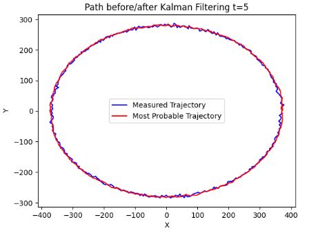
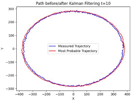
- The above plots confirm that KF is well suited to sparse input and state tracking.
- It is shown that reasonable estimates of a circular trajectory can be accomplished.
- The crucial point is that the measurement and state prediction error parameters (noise parameters) are learned solely from the available data (stored in the kalmann0.txt file).
- Example 2: We apply the Extended Kalman Filter (EKF) to a circular motion robot. The objective is to study the impact of a position error std (denoted by sigma) on the accuracy of KF predictions.
- Business value: A KF approach to reduce position error for pedestrian applications in areas of bad GPS reception.
#https://github.com/NeerajSakethVamsi/Localization_KalmanFilter/blob/main/extended_kalmanfilter_circularmotion.py
import numpy as np
import matplotlib.pyplot as plt
import math

class Filter:
    def __init__(self, var=None):
        self.filter = var
        self.filter.predict()

    def get_point(self):
        return self.filter.x[0:2].flatten()

    def predict_point(self, measurement):

        self.filter.predict()
        self.filter.update(measurement)
        return self.get_point()


class ExtendedKalmanFilter:
    def __init__(self,sigma,u,dt):
        self.x = np.array([0.,  # x
                           0.,  # y
                           0.,  # orientation
                           0.]).reshape(-1, 1)  # linear velocity

        self.u = u
        self.dt = dt
        self.p = np.diag([999. for i in range(4)])
        self.q = np.diag([0.1 for i in range(4)])
        self.r = np.diag([sigma, sigma])
        self.jf = np.diag([1. for i in range(4)])
        self.jg = np.array([[1., 0., 0., 0.],
                            [0., 1., 0., 0.]])
        self.h = np.array([[1., 0., 0., 0.],
                           [0., 1., 0., 0.]])
        self.z = np.array([0.,
                           0.]).reshape(-1, 1)

    def predict(self):
        x, y, phi, v = self.x
        vt, wt = self.u
        dT = self.dt

        new_x = x + vt * np.cos(phi) * dT
        new_y = y + vt * np.sin(phi) * dT
        new_phi = phi + wt * dT
        new_v = vt

        self.x[0]=new_x
        self.x[1]=new_y
        self.x[2]=new_phi
        self.x[3]=new_v

        self.jf[0][2] = -v * np.sin(phi) * dT
        self.jf[0][3] = v * np.cos(phi) * dT
        self.jf[1][2] = v * np.cos(phi) * dT
        self.jf[1][3] = v * np.sin(phi) * dT

        # p-prediction:
        self.p = self.jf.dot(self.p).dot(self.jf.transpose()) + self.q

    def update(self, measurement):
        z = np.array(measurement).reshape(-1, 1)
        y = z - self.h.dot(self.x)

        s = self.jg.dot(self.p).dot(self.jg.transpose()) + self.r
        k = self.p.dot(self.jg.transpose()).dot(np.linalg.inv(s))

        self.x = self.x + k.dot(y)
        self.p = (np.eye(4) - k.dot(self.h)).dot(self.p)

def action(parfilter, measurements):
    result = []
    for i in range(len(measurements)):
        m = measurements[i]
        pred = parfilter.predict_point(m)
        result.append(pred)

    return result

def create_artificial_circle_data(radius,dt,u,sigma):
    measurements = []
    vt, wt = u
    phi = np.arange(0, 2*math.pi, wt * dt)
    x = radius * np.cos(phi) + sigma * np.random.randn(len(phi))
    y = radius * np.sin(phi) + sigma * np.random.randn(len(phi))

    measurements += [[x, y] for x, y in zip(x, y)]
    return measurements

def plot(measurements, result, deadreckon_results):
    plt.figure("Extended Kalman Filter Visualization")
    plt.scatter([x[0] for x in measurements], [x[1] for x in measurements], c='red', label='GPS Position', alpha=0.3,s=4)
    plt.scatter([x[0] for x in result], [x[1] for x in result], c='blue', label='Kalman filter estimate Position', alpha=0.3, s=4,marker='x')
    plt.scatter([x[0] for x in deadreckon_results], [x[1] for x in deadreckon_results], c='black', label='dead reckoning Position', alpha=0.3, s=4,marker='x')
    plt.legend()
    plt.grid('on')
    plt.title("Circular Motion Robot and Kalman Filter Prediction sigma=0.1")
    plt.xlabel("X-axis")
    plt.ylabel("Y-axis")
    plt.xlim(-10, 10)
    plt.ylim(-10, 10)
    plt.tight_layout()
    plt.show()

def deadReckoning(robo, u, dt):
    initial_state = robo.x
    vt, wt = u
    x=vt/wt
    y=0
    phi=math.pi/2
    x_list=[]
    y_list=[]
    phi_list=[]
    result = []
    T = 2 * math.pi / wt
    for i in range(int(T/dt)):
        new_x = x + vt * np.cos(phi) * dt
        new_y = y + vt * np.sin(phi) * dt
        new_phi = phi + wt * dt
        x = new_x
        y = new_y
        phi = new_phi
        # new_v = vt

        x_list.append(new_x)
        y_list.append(new_y)
        phi_list.append(new_phi)
    result += [[p, q] for p, q in zip(x_list, y_list)]

    return result

if __name__ == '__main__':
    input_u = [10, 2]
    radiusOfCircle = input_u[0] / input_u[1]
    robot = ExtendedKalmanFilter(sigma=0.1, u=input_u, dt=0.001)
    robotController = Filter(robot)
    deadreckon_results=deadReckoning(robo=robot, u=input_u, dt=0.001)
    measurementGPS = create_artificial_circle_data(radius=radiusOfCircle,u=input_u, dt=0.001, sigma=0.1)
    results = action(robotController, measurementGPS)
    plot(measurementGPS, results, deadreckon_results)

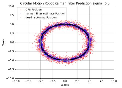


- These plots show that the EKF prediction of the system state does handle well even the highly erroneous position measurements.
- Indeed, EKF can be used to improve the accuracy of GPS by providing more precise position coordinates and reducing errors.
2D Location Tracking
- Let’s discuss the implementation of KF for tracking a moving object in 2D direction.
- Example 1: KF Model for Airplane movement in XY Direction.
import numpy as np
import matplotlib.pyplot as plt
import seaborn as sb
itr = 50

# Initial Observations
ini_Vx = 25 # m/s
ini_Vy = 15 # m/s
ini_X = 150 # m
ini_Y = 280 # m
ini_observation = np.array([ini_X, ini_Y, ini_Vx, ini_Vy])

# Assuming accelaration is constant
ini_Ax = 2 # m/s²
ini_Ay = 1 # m/s²
ini_accelaration = np.array([ini_Ax, ini_Ay])

# Process errors in Process Covariance Matrix (Error due to machine or any other process in calculations)
del_PX = 20 # m  20   40
del_PY = 15 # m   15  30
del_PVx = 5 # m/s   5   10
del_PVy = 3.5 # m/s  3.5 7
process_errors = np.array([del_PX, del_PY, del_PVx, del_PVy])

# Observation errors
del_X = 25 # 25
del_Y = 18 # 18 m
del_Vx = 6 # 6 m/s
del_Vy = 5 # 5 m/s
observation_errors = np.array([del_X, del_Y, del_Vx, del_Vy])

# Time difference between each ebservation
del_T = 1 # s
#Write down Observed State matrix.
X = np.array([ini_observation])

# Generate Position Vectors based on velocity vector
for i in range(1,itr+1):
    perfVx = ini_Vx + ini_Ax*i*del_T
    perfVy = ini_Vy + ini_Ay*i*del_T
    perfX = X[i-1][0] + perfVx
    perfY = X[i-1][1] + perfVy

    random_Vx_err = np.random.uniform(-del_Vx, del_Vx, size=1)
    random_Vy_err = np.random.uniform(-del_Vy, del_Vy, size=1)
    random_X_err = np.random.uniform(-del_X, del_X, size=1)
    random_Y_err = np.random.uniform(-del_Y, del_Y, size=1)

    X = np.append(X, [[perfX+random_X_err[0], perfY+random_Y_err[0], perfVx+random_Vx_err[0], perfVy+random_Vy_err[0]]], axis=0)
#Generate A and B matrices according to shape of state matrix.

# A matrix
A = np.array([[1, 0, del_T, 0],
              [0, 1, 0, del_T],
              [0, 0, 1, 0],
              [0, 0, 0, 1]])

# B matrix
B = np.array([[(del_T**2)*0.5, 0],
              [0, (del_T**2)*0.5],
              [del_T, 0],
              [0, del_T]])
#Function to generate covariance matrix
def generate_Covariance(dim, errors):
    cov_mat = errors**2 * np.identity(dim)
    # print(cov_mat)
    return cov_mat
#Calculate Measurement Noice Covariance matrix R, Process Noice Covariance matrix Q and State Covariance Matrix P.
# R = Measurement Covariance Matrix --> Error in the measurement
# Needs to generate only once in whole process
R = generate_Covariance(observation_errors.shape[0], observation_errors)
# print(R)

# Q = Process Covariance Matrix --> Error in the process
Q = generate_Covariance(process_errors.shape[0], process_errors)
print(process_errors)
print(Q)

# P = State Covariance Matrix --> Error in the estimate
P = generate_Covariance(process_errors.shape[0], process_errors)

# Let's keep P and Q keep same in first iteration
# Q will be constant in every iteration, but P will change

[20.  15.   5.   3.5]
[[400.     0.     0.     0.  ]
 [  0.   225.     0.     0.  ]
 [  0.     0.    25.     0.  ]
 [  0.     0.     0.    12.25]]
#Define function to calculate Normal Distribution

def Normal_Distribution(prev_state, mean, variance):
    ans = []

    for ix in range(variance.shape[0]):
        for iy in range(variance.shape[1]):
            if ix==iy:
                value = (1 / (np.sqrt(variance[ix][iy]*2*np.pi))) * np.exp(-0.5 * (np.square(prev_state[ix]-mean)/variance[ix][iy]))
                ans.append(value)

    return np.array(ans)
#Function to predict state

Uk = np.array([ini_Ax, ini_Ay])

# Assuming their is no noice
def predict_state(A, B, prev_state, W):
    curr_state = np.matmul(A, prev_state) + np.matmul(B, Uk) + W
    curr_state = np.array(curr_state)

    return curr_state
#Function to generate Predicted Process Covariance Matrix
# This function will run only  one time, on 1st iteration
def predict_process_covariance(first_PC, A, Q):
    predicted_P = np.matmul(A, np.matmul(first_PC, np.transpose(A))) + Q

    # Make predicted_P a diagonal Matrix
    predicted_P = np.multiply(predicted_P, np.identity(predicted_P.shape[0]))
    return predicted_P
#Update Process Covariance Matrix
def update_proccess_covariance(prev_PC, K):
    updated_PC = (np.identity(K.shape[0]) - K) * prev_PC

    return updated_PC
#Function to calculate Kalman Gain.
def Kalman_Gain(predicted_P, R):
    if predicted_P.shape == R.shape:
        K = np.divide(predicted_P, predicted_P + R, where = predicted_P!=0)

    # Make K a diagonal Matrix
    K = np.multiply(K, np.identity(K.shape[0]))
    return K
#Function to calculate new observation Y.
def new_Observation(observed_state, V):
    Y = observed_state + V
    return Y
#Function to calculate next state based on Kalman Gain.
def generate_State(curr_state_equ, K, new_Obs):
    predicted_state = curr_state_equ + np.matmul(K, new_Obs - curr_state_equ)
    return predicted_state
#Final Loop for itr Iterations.
final_prediction = np.array([X[0]])
final_observation = np.array([])
final_calculated = np.array([])

for curr_itr in range(itr):

    # Calculating W and V for current iteration
    W = Normal_Distribution(X[curr_itr], 0, Q)
    V = Normal_Distribution(X[curr_itr], 0, R)

    if curr_itr == 0:
        # Calculating State
        curr_state = predict_state(A, B, X[curr_itr], W)
        final_calculated = np.append(final_calculated, curr_state)
        curr_P = predict_process_covariance(P, A, Q)

        # Calculate Kalman Gain
        curr_KGain = Kalman_Gain(curr_P, R)

        # Calculate new observation Y
        new_Obs = new_Observation(X[curr_itr], V)
        final_observation = np.append(final_observation, new_Obs)

        # Calculate new Predicted state based on Kalman Gain calculations
        predicted_state = generate_State(curr_state, curr_KGain, new_Obs)
        # final_prediction = np.append(final_prediction, predicted_state)

        # Calculate new Process Covariance Matrix
        updated_PC = update_proccess_covariance(curr_P, curr_KGain)

    else:
        curr_state = predict_state(A, B, prev_state, W)
        final_calculated = np.append(final_calculated, curr_state)

        curr_P = predict_process_covariance(prev_PC, A, Q)
        curr_KGain = Kalman_Gain(curr_P, R)

        # new_Obs = new_Observation(X[curr_itr+1], V)
        new_Obs = X[curr_itr]
        final_observation = np.append(final_observation, new_Obs)

        predicted_state = generate_State(curr_state, curr_KGain, new_Obs)
        final_prediction = np.append(final_prediction, predicted_state)

        updated_PC = update_proccess_covariance(curr_P, curr_KGain)

    prev_state = predicted_state
    prev_PC = updated_PC
finali = []
for i in range(int(final_prediction.shape[0]/4)):
    tempi = []
    for j in range( 4*i , 4*i + 4 ):
        tempi.append(final_prediction[j])
    finali.append(tempi)


finali = np.array(finali)
final0 = []
for i in range(int(final_observation.shape[0]/4)):
    temp0 = []
    for j in range(4*i, 4*i + 4):
        temp0.append(final_observation[j])
    final0.append(temp0)


final0 = np.array(final0)
finalc = []
for i in range(int(final_calculated.shape[0]/4)):
    tempc = []
    for j in range(4*i, 4*(i+1)):
        tempc.append(final_calculated[j])
    finalc.append(tempc)

finalc = np.array(finalc)
plt.figure(figsize=(12,8))
plt.plot(finalc[:15,0], finalc[:15,1], label="Observed")
plt.plot(finali[:15,0], finali[:15,1], label="Calculated")
plt.plot(final0[:15,0], final0[:15,1], label="Predicted")
plt.legend()
plt.title("Test 1: dX=25 dY=18 dVx=6 dVy=5")
plt.xlabel("Position X (in m)")
plt.ylabel("Position Y (in m)")
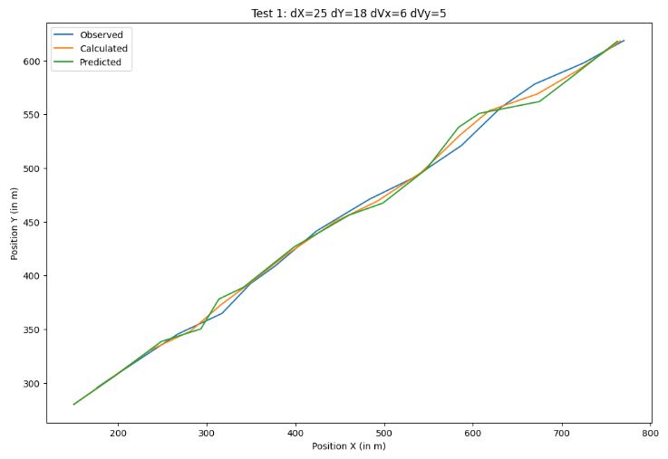


Notations: (dX, dY) = (XY) position error, (dVx, dVy) = (XY) velocity vector error, e.g.
# Observation errors
del_X = 25 # 25
del_Y = 18 # 18 m
del_Vx = 6 # 6 m/s
del_Vy = 5 # 5 m/s
- The above tests have been performed using the following input process errors
# Process errors in Process Covariance Matrix (Error due to machine or any other process in calculations)
del_PX = 20 # m  20   40
del_PY = 15 # m   15  30
del_PVx = 5 # m/s   5   10
del_PVy = 3.5 # m/s  3.5 7


- Tests 1-5 confirm the robustness of KF-based 2D object tracking against uncertainties in process and measurement noise covariances. It is shown that KF is robust enough if the process and measurement noise covariances are changed. It appears that KF gains can be insensitive to scaling of covariance matrices.
- Example 2: Sensing and planning for Autonomous vehicles by implementing the Extended Kalman Filter (EKF) for Lidar and Radar data.
#Importing libraries
import numpy as np
from sympy import Symbol, symbols, Matrix, sin, cos, sqrt
from sympy import init_printing
import matplotlib.pyplot as plt
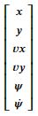
vx, vy, psis, dpsis, dts, xs, ys = symbols('vx vy \psi \dot\psi T x y')

# desired state vector
number_of_states = 6
state = Matrix([xs,ys,vx,vy,psis,dpsis])
state
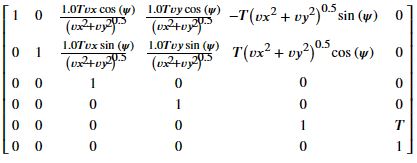
# constant turn rate and constant velocity non linear plant model
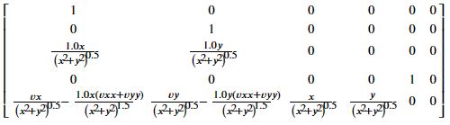
gs = Matrix([[xs+((vx**2 + vy**2)**0.5)*(cos(psis))*dts],
[ys+((vx**2 + vy**2)**0.5)*(sin(psis))*dts],
[vx],
[vy],
[psis+dpsis*dts],
[dpsis]])
gs

gs.jacobian(state)
# from data analysis
dt = 1.0/10.0  # Sample Rate is 10Hz

# Inital Uncertainity matrix
P = np.diag([1000.0, 1000.0, 1000.0, 1000.0, 1000.0, 1000.0])
print(P)

# Process Noise Covariance Matrix
sPos = 0.5*5*dt**2  # assume 5m/s2 as maximum acceleration, forcing the vehicle
sYaw = 0.1*dt         # assume 0.1rad/s as maximum turn rate for the vehicle
sVel = 5*dt         # assume 5m/s2 as maximum acceleration, forcing the vehicle
sYawRate = 1*dt         # assume 1.0rad/s2 as the maximum turn rate acceleration for the vehicle

Q = np.diag([sPos**2, sPos**2, sVel**2, sVel**2, sYaw**2, sYawRate**2])

# measurement covariance matrix
R = np.matrix([[0.01, 0.0, 0.0, 0.0, 0.0],
               [0.0, 0.01, 0.0, 0.0, 0.0],
               [0.0, 0.0, 0.01, 0.0, 0.0],
               [0.0, 0.0, 0.0, 1.0e-2, 0.0],
               [0.0, 0.0, 0.0, 0.0, 0.01]])

[[1000.    0.    0.    0.    0.    0.]
 [   0. 1000.    0.    0.    0.    0.]
 [   0.    0. 1000.    0.    0.    0.]
 [   0.    0.    0. 1000.    0.    0.]
 [   0.    0.    0.    0. 1000.    0.]
 [   0.    0.    0.    0.    0. 1000.]]
## measurement vector
hs = Matrix([[xs],
             [ys],
             [(xs**2 + ys**2)**0.5],
             [psis],
             [(xs*vx + ys*vy)/(xs**2 + ys**2)**0.5]])
hs

## Jacobian of hs
hs.jacobian(state)
## data parser

class DataPoint:
  """
    A set of derived information from measurements of known sensors
    NOTE: Upon instantiation of a "radar" DataPoint, state variables are computed from raw data
  """

  def __init__(self, d):
    self.timestamp = d['timestamp']
    self.name = d['name']
    self.all = d
    self.raw = []
    self.data = []

    if self.name == 'state':
      self.data = [d['x'], d['y'], d['vx'], d['vy'], d['yaw'], d['yaw_rate']]
      self.raw = self.data.copy()

    elif self.name == 'lidar':
      self.data = [d['x'], d['y'], 0, 0, 0]
      self.raw = [d['x'], d['y']]

    elif self.name == 'radar':
      self.data = [0, 0, d['rho'], d['phi'], d['drho']]
      self.raw = [d['rho'], d['phi'], d['drho']]

    self.all['processed_data'] = self.data
    self.all['raw'] = self.raw

  def get_dict(self):
    return self.all

  def get_raw(self):
    return self.raw

  def get(self):
    return self.data

  def get_timestamp(self):
    return self.timestamp

  def get_name(self):
    return self.name

def parse_data(file_path):

  all_sensor_data = []
  all_ground_truths = []

  with open(file_path) as f:

    for line in f:
      data = line.split()

      if data[0]  == 'L':

        sensor_data = DataPoint({
          'timestamp': int(data[3]),
          'name': 'lidar',
          'x': float(data[1]),
          'y': float(data[2])
        })

        g = {'timestamp': int(data[3]),
             'name': 'state',
             'x': float(data[4]),
             'y': float(data[5]),
             'vx': float(data[6]),
             'vy': float(data[7]),
             'yaw' : float(data[8]),
             'yaw_rate' : float(data[9])
        }

        ground_truth = DataPoint(g)

      elif data[0] == 'R':

        sensor_data = DataPoint({
          'timestamp': int(data[4]),
          'name': 'radar',
          'rho': float(data[1]),
          'phi': float(data[2]),
          'drho': float(data[3])
        })

        g = {'timestamp': int(data[4]),
             'name': 'state',
             'x': float(data[5]),
             'y': float(data[6]),
             'vx': float(data[7]),
             'vy': float(data[8]),
             'yaw' : float(data[9]),
             'yaw_rate' : float(data[10])
        }
        ground_truth = DataPoint(g)

      all_sensor_data.append(sensor_data)
      all_ground_truths.append(ground_truth)

  return all_sensor_data, all_ground_truths

all_sensor_data, all_ground_truths = parse_data("./data_ekf.txt")

# desired state vector
number_of_states = 6
# initial state i.e. x[0]
x = np.matrix([[1, 1, 1, 1, 1, 1]]).T
I = np.eye(number_of_states)
all_estimations = []

# from data analysis
dt = 1.0/10.0  # Sample Rate is 10Hz

for filterstep in range(len(all_sensor_data)):

  # Prediction
  x[0] = dt * (np.sqrt(x[2] ** 2 + x[3] ** 2)) * np.cos(x[4]) + x[0]
  x[1] = dt * (np.sqrt(x[2] ** 2 + x[3] ** 2)) * np.sin(x[4]) + x[1]
  x[2] = x[2]
  x[3] = x[3]
  x[4] = dt * x[5] + x[4]
  x[5] = x[5]

  # Calculate the Jacobian of the Dynamic Matrix A
  a02 = float((dt * x[2] * np.cos(x[4])) / (np.sqrt(x[2] ** 2 + x[3] ** 2)))
  a03 = float((dt * x[3] * np.cos(x[4])) / (np.sqrt(x[2] ** 2 + x[3] ** 2)))
  a12 = float((dt * x[2] * np.sin(x[4])) / (np.sqrt(x[2] ** 2 + x[3] ** 2)))
  a13 = float((dt * x[3] * np.sin(x[4])) / (np.sqrt(x[2] ** 2 + x[3] ** 2)))
  a04 = float(-dt*(np.sqrt(x[2] ** 2 + x[3] ** 2)) * np.sin(x[4]))
  a14 = float(-dt*(np.sqrt(x[2] ** 2 + x[3] ** 2)) * np.cos(x[4]))

  JA = np.matrix([[1.0, 0.0, a02, a03, a04, 0.0],
                  [0.0, 1.0, a12, a13, a14, 0.0],
                  [0.0, 0.0, 1.0, 0.0, 0.0, 0.0],
                  [0.0, 0.0, 0.0, 1.0, 0.0, 0.0],
                  [0.0, 0.0, 0.0, 0.0, 1.0, dt],
                  [0.0, 0.0, 0.0, 0.0, 0.0, 1.0]])

  # Project the error covariance ahead
  P = JA*P*JA.T + Q

  # Measurement Update (Correction) & Kalman Gain
  hx = np.matrix([[float(x[0])],
                  [float(x[1])],
                  [float(np.sqrt(x[0]**2 + x[1]**2))],
                  [float(x[4])],
                  [float((x[2]*x[0] + x[3]*x[1])/(np.sqrt(x[0] ** 2 + x[1] ** 2)))]])

  if all_sensor_data[filterstep].get_name() == 'lidar':
    JH = np.matrix([[1.0, 0.0, 0.0, 0.0, 0.0, 0.0],
                   [0.0, 1.0, 0.0, 0.0, 0.0, 0.0],
                   [0.0, 0.0, 0.0, 0.0, 0.0, 0.0],
                   [0.0, 0.0, 0.0, 0.0, 0.0, 0.0],
                   [0.0, 0.0, 0.0, 0.0, 0.0, 0.0]])
  else:
    h20 = float(x[0]/(np.sqrt(x[0] ** 2 + x[1] ** 2)))
    h21 = float(x[1]/(np.sqrt(x[0] ** 2 + x[1] ** 2)))
    h40 = float((x[2] / (np.sqrt(x[0] ** 2 + x[1] ** 2))) - ((x[0] * (x[0]*[2] + x[1]*x[3])) / (np.power((x[0] ** 2 + x[1] ** 2), 1.5))))
    h41 = float((x[3] / (np.sqrt(x[0] ** 2 + x[1] ** 2))) - ((x[1] * (x[0]*[2] + x[1]*x[3])) / (np.power((x[0] ** 2 + x[1] ** 2), 1.5))))
    h42 = float(x[0]/np.sqrt(x[0] ** 2 + x[1] ** 2))
    h43 = float(x[1]/np.sqrt(x[0] ** 2 + x[1] ** 2))

    JH = np.matrix([[0.0, 0.0, 0.0, 0.0, 0.0, 0.0],
                    [0.0, 0.0, 0.0, 0.0, 0.0, 0.0],
                    [h20, h21, 0.0, 0.0, 0.0, 0.0],
                    [0.0, 0.0, 0.0, 0.0, 1.0, 0.0],
                    [h40, h41, h42, h43, 0.0, 0.0]])

  S = JH*P*JH.T + R
  K = (P*JH.T) * np.linalg.inv(S)

  # Update the estimate via
  Z = np.array(all_sensor_data[filterstep].get_dict()['processed_data']).reshape(JH.shape[0],1)
  y = Z - (hx)
  x = x + (K*y)

  # Update the error covariance
  P = (I - (K*JH))*P

  # save states for analysis
  all_estimations.append(x.reshape(-1).tolist())
ground = []
for i in range(len(all_ground_truths)):
  ground.append(all_ground_truths[i].get())

ground = np.array(ground)
all_estimations = np.array(all_estimations)
all_estimations = all_estimations.reshape(500,-1)
print(all_estimations.shape)
plt.plot(all_estimations[:, 0], all_estimations[:,1],label = "estimate")
plt.plot(ground[:,0],ground[:,1],label = "ground")
plt.xlabel('X')
plt.ylabel('Y')
plt.title('Test 3: R=0.01*diag(1,1,1,1,1)')
plt.legend()
plt.show()

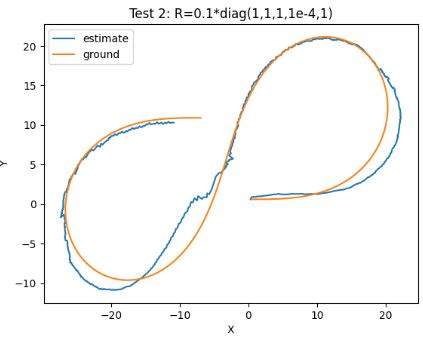

- These three tests confirm that EKF is not too sensitive to the measurement covariance matrix R with inherent uncertainty.
- The observed numerical stability of EKF makes it feasible for practical usage in cases of real time applications.
3D Location Tracking
- Let’s walk through the KF-based single ball 3D tracking algorithm.
- Input parameters: position and velocity at start, the drag resistance coefficient, and damping.
- Measurements: 200 data points with random noise.
#Import basic libraries
import numpy as np
%matplotlib inline
import matplotlib.pyplot as plt
from scipy.stats import norm
#Initial data
# Time step
dt = 0.01

# total number of measurements
m = 200
# positions at start
px= 0.0
py= 0.0
pz= 1.0

# velocities at start
vx = 5.0
vy = 3.0
vz = 0.0

# Drag Resistance Coefficient
c = 0.1

# Damping
d = 1.9

# Arrays to store location measurements
Xr=[]
Yr=[]
Zr=[]
#Measurements
# generating data
for i in range(0, m):

 # update acceleration (deceleration), velocity, position in x direction
    accx = -c*vx**2
    vx += accx*dt
    px += vx*dt
 # update acceleration (deceleration), velocity, position in y direction
    accy = -c*vy**2
    vy += accy*dt
    py += vy*dt
 # update acceleration, velocity, position in x direction
    accz = -9.806 + c*vz**2
    vz += accz*dt
    pz += vz*dt
 # if the object is about to hit the base,
 # change direction, with damping
    if pz<0.01:
        vz=-vz*d
        pz+=0.02
 # add to the arrays storing locations
    Xr.append(px)
    Yr.append(py)
    Zr.append(pz)
# Add random noise to measurements
# Standard Deviation for noise
sp= 0.4
Xm = Xr + sp * (np.random.randn(m))
Ym = Yr + sp * (np.random.randn(m))
Zm = Zr + sp * (np.random.randn(m))
# stack the measurements together for ease of later use
measurements = np.vstack((Xm,Ym,Zm))
fig = plt.figure(figsize=(10,6))
Three_dplot = fig.add_subplot(111, projection='3d')
Three_dplot.scatter(Xm, Ym, Zm, c='red')
Three_dplot.set_xlabel('$x$')
Three_dplot.set_ylabel('$y$')
Three_dplot.set_zlabel('$z$')
plt.title('Noisy 3D Ball-Location observations noise 40%')
plt.show()


# Identity matrix
I = np.eye(9)

# state matrix
x = np.matrix([0.0, 0.0, 1.0, 5.0, 3.0, 0.0, 0.0, 0.0, -9.81]).T

# P matrix
P = 100.0*np.eye(9)
# A matrix
A = np.matrix([[1.0, 0.0, 0.0, dt, 0.0, 0.0, 1/2.0*dt**2, 0.0, 0.0],
 [0.0, 1.0, 0.0, 0.0, dt, 0.0, 0.0, 1/2.0*dt**2, 0.0],
 [0.0, 0.0, 1.0, 0.0, 0.0, dt, 0.0, 0.0, 1/2.0*dt**2],
 [0.0, 0.0, 0.0, 1.0, 0.0, 0.0, dt, 0.0, 0.0],
 [0.0, 0.0, 0.0, 0.0, 1.0, 0.0, 0.0, dt, 0.0],
 [0.0, 0.0, 0.0, 0.0, 0.0, 1.0, 0.0, 0.0, dt],
 [0.0, 0.0, 0.0, 0.0, 0.0, 0.0, 1.0, 0.0, 0.0],
 [0.0, 0.0, 0.0, 0.0, 0.0, 0.0, 0.0, 1.0, 0.0],
 [0.0, 0.0, 0.0, 0.0, 0.0, 0.0, 0.0, 0.0, 1.0]])
# H matrix
H = np.matrix([[1.0, 0.0, 0.0, 0.0, 0.0, 0.0, 0.0, 0.0, 0.0],
 [0.0, 1.0, 0.0, 0.0, 0.0, 0.0, 0.0, 0.0, 0.0],
 [0.0, 0.0, 1.0, 0.0, 0.0, 0.0, 0.0, 0.0, 0.0]])

# R matrix
r = 1.0
R = np.matrix([[r, 0.0, 0.0],
 [0.0, r, 0.0],
 [0.0, 0.0, r]])

# Q, G matrices
s = 8.8
G = np.matrix([[1/2.0*dt**2],
 [1/2.0*dt**2],
 [1/2.0*dt**2],
 [dt],
 [dt],
 [dt],
 [1.0],
 [1.0],
 [1.0]])
Q = G*G.T*s**2
B = np.matrix([[0.0], #Disturbance Control Matrix
               [0.0],
               [0.0],
               [0.0],
               [0.0],
               [0.0],
               [0.0],
               [0.0],
               [0.0]])
u = 0.0 #Control Input
#Initialization
xt = []
yt = []
zt = []
dxt= []
dyt= []
dzt= []
ddxt=[]
ddyt=[]
ddzt=[]
Zx = []
Zy = []
Zz = []
Px = []
Py = []
Pz = []
Pdx= []
Pdy= []
Pdz= []
Pddx=[]
Pddy=[]
Pddz=[]
Kx = []
Ky = []
Kz = []
Kdx= []
Kdy= []
Kdz= []
Kddx=[]
Kddy=[]
Kddz=[]
onFloor = False
for i in range(0, m):
# Model the direction switch, when hitting the plate
    if x[2]<0.02 and not onFloor:
        x[5] = -x[5]
        onFloor=True
# Prediction
# state prediction
    x = A*x + B*u
# Project the error covariance ahead
    P = A*P*A.T + Q
# Update
# Kalman Gain
    S = H*P*H.T + R
    K = (P*H.T) * np.linalg.pinv(S)
# Update the estimate via z
    Z = measurements[:,i].reshape(H.shape[0],1)
    y = Z - (H*x)
    x = x + (K*y)
# error covariance
    P = (I - (K*H))*P

    # Storing results
    xt.append(float(x[0]))
    yt.append(float(x[1]))
    zt.append(float(x[2]))
    dxt.append(float(x[3]))
    dyt.append(float(x[4]))
    dzt.append(float(x[5]))
    ddxt.append(float(x[6]))
    ddyt.append(float(x[7]))
    ddzt.append(float(x[8]))
    Zx.append(float(Z[0]))
    Zy.append(float(Z[1]))
    Zz.append(float(Z[2]))
    Px.append(float(P[0,0]))
    Py.append(float(P[1,1]))
    Pz.append(float(P[2,2]))
    Pdx.append(float(P[3,3]))
    Pdy.append(float(P[4,4]))
    Pdz.append(float(P[5,5]))
    Pddx.append(float(P[6,6]))
    Pddy.append(float(P[7,7]))
    Pddz.append(float(P[8,8]))
    Kx.append(float(K[0,0]))
    Ky.append(float(K[1,0]))
    Kz.append(float(K[2,0]))
    Kdx.append(float(K[3,0]))
    Kdy.append(float(K[4,0]))
    Kdz.append(float(K[5,0]))
    Kddx.append(float(K[6,0]))
    Kddy.append(float(K[7,0]))
    Kddz.append(float(K[8,0]))
# Plots
#State Estimates
plt.figure(figsize=(12,6))
plt.subplot(311)
plt.title('Location, Velocity, Acceleration Estimates Noise 40%')
plt.plot(range(len(measurements[0])),xt, label='$x$')
plt.plot(range(len(measurements[0])),yt, label='$y$')
plt.plot(range(len(measurements[0])),zt, label='$z$')
plt.legend(loc='right' )
plt.figure(figsize=(12,6))

plt.subplot(312)
plt.plot(range(len(measurements[0])),dxt, label='$v_x$')
plt.plot(range(len(measurements[0])),dyt, label='$v_y$')
plt.plot(range(len(measurements[0])),dzt, label='$v_z$')
plt.legend(loc='right')
plt.subplot(313)
plt.plot(range(len(measurements[0])),ddxt, label='$ax$')
plt.plot(range(len(measurements[0])),ddyt, label='$ay$')
plt.plot(range(len(measurements[0])),ddzt, label='$az$')
plt.legend(loc='right')
plt.xlabel('Step')
- Location estimates noise 20%

- Velocity, acceleration estimates noise 20%

- Location estimates noise 40%

- Velocity, acceleration estimates noise 40%

# Location in 2D (z, y)
plt.figure(figsize=(12,6))
plt.subplot(311)
plt.plot(xt,yt, label='Estimate')
plt.scatter(Xm,Ym, label='Measurement', c='red', s=30)
plt.plot(Xr, Yr, label='Real d=1.9')
plt.title('Location Tracking on the 2D-Planes')
plt.legend(loc='best')
plt.xlabel('$x$')
plt.ylabel('$y$')
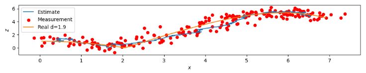
plt.figure(figsize=(12,6))
plt.subplot(312)
plt.plot(xt,zt, label='Estimate')
plt.scatter(Xm,Zm, label='Measurement', c='red', s=30)
plt.plot(Xr, Zr, label='Real d=1.9')
plt.legend(loc='best')
plt.xlabel('$x$')
plt.ylabel('$z$')
plt.figure(figsize=(12,6))
plt.subplot(313)
plt.plot(yt,zt, label='Estimate')
plt.scatter(Ym,Zm, label='Measurement', c='red', s=30)
plt.plot(Yr, Zr, label='Real d=0.9')
plt.legend(loc='best')
plt.axhline(0, color='k')
plt.xlabel('$y$')
plt.ylabel('$z$')
# Location in 3D (X, Y, Z)
fig = plt.figure(figsize=(16,9))
ax = fig.add_subplot(111, projection='3d')
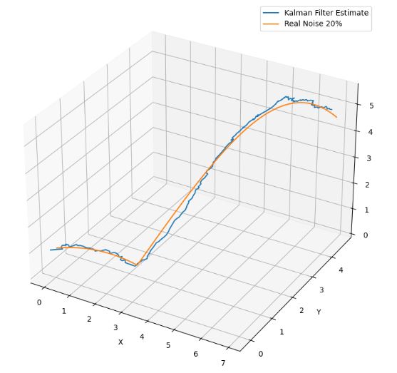
ax.plot(xt,yt,zt, label='Kalman Filter Estimate')
ax.plot(Xr, Yr, Zr, label='Real Noise 40%')
ax.set_xlabel('X')
ax.set_ylabel('Y')
ax.set_zlabel('Z')
ax.legend()
- Location Tracking on the 2D-Plane (XY) Noise 20%
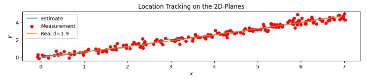
- Location Tracking on the 2D-Plane (XY) Noise 40%

- Location Tracking on the 2D-Plane (XZ) Noise 20%

- Location Tracking on the 2D-Plane (XZ) Noise 40%
- Location Tracking on the 2D-Plane (YZ) Noise 20%

- Location Tracking on the 2D-Plane (YZ) Noise 40%

- Location Tracking in 3D Space Noise 20%
- Location Tracking in 3D Space Noise 40%

- These plots confirm that a larger noise-to-signal ratio (N/S) does not cause a serious degradation in 3-D ball trajectory estimation using the proposed KF approach.
- The measurement equation is obtained by analyzing the effect of white Gaussian noise on 3-D positional errors.
- Simulation results indicate that the KF equations derived in this experiment represent an accurate model for 3-D motion estimation in spite of the aforementioned assumptions used in the derivation.
Summary
- In this post, we have addressed the problem of object tracking used in video surveillance, car/airplane/drone/human/ball tracking, etc.
- KF is especially convenient for objects which motion model is known, plus they incorporate some extra information in order to estimate the next object position more robustly.
- If we have a linear motion model, and process and measurement noise are Gaussian-like, then KF represents the optimal solution for the state update (in our case tracking problem).
- Results have shown that both KF and EKF don’t introduce large errors in the estimated parameters when the N/S ratio is not small.
- In this study, we have focused on the problem of a single object tracking. The issues of tracking multiple objects simultaneously will be studied elsewhere.
Explore More
- Kalman-Based Target Trajectory Tracking Performance QC Analysis
- Anatomy of the Robust 1D Kalman Filter
References
- An Introduction to the Kalman Filter
- Robust Kalman filtering for discrete-time nonlinear systems with parameter uncertainties
- Position and Velocity Estimations of 2D-Moving Object Using Kalman Filter: Literature Review
- Estimation of angular velocity and acceleration with Kalman filter, based on position measurement only
- Kalman Filter estimation of angular acceleration
- A Study on Real Time Circular Motion in Robots Using Kalman Filters
- Estimation for Motion in Tracking and Detection Objects with Kalman Filter
- Single View Ball Tracking and 3D Trajectory Reconstruction in Basketball Videos


One-Time
Monthly
Yearly
Make a one-time donation
Make a monthly donation
Make a yearly donation
Choose an amount
€5.00
€15.00
€100.00
€5.00
€15.00
€100.00
€5.00
€15.00
€100.00
Or enter a custom amount
€
Your contribution is appreciated.
Your contribution is appreciated.
Your contribution is appreciated.
DonateDonate monthlyDonate yearly
Leave a comment