
The featured image was created in Canva.
- The objective of this post is to extend our previous studies by applying PCA, T-SNE and tuned supervised Machine Learning (ML) algorithms to malware (malicious software) detection & interpretation.
- Part 1: We will use the Benign & Malicious PE Files dataset to evaluate the malware binary classification clustering approach vs simple ML antimalware in Python.
- Part 2: We will also investigate the behavior of KPIs specific to the Decision Tree (DT) model and arising when the metrics are computed on validation data.
- Scope: We will re-implement these open-source techniques while comparing them against the same benchmark data.
- Motivation: Detection of unknown malware has been a challenge to businesses, governments and end-users. The dependency on signature-based detection has proven to be inefficient. Recent R&D studies revealed that AI can impact cybersecurity throughout it’s entire life cycle, yielding benefits like automation, threat intelligence, and improved cyber defense.
Input Data
- Setting the working directory YOURPATH
import os
os.chdir('YOURPATH')    # Set working directory
os. getcwd()
- Importing the basic libraries and reading the input Kaggle dataset
import numpy as np # linear algebra
import pandas as pd # data processing, CSV file I/O (e.g. pd.read_csv)
df0=pd.read_csv('dataset_malwares.csv')
df0.columns
Index(['Name', 'e_magic', 'e_cblp', 'e_cp', 'e_crlc', 'e_cparhdr',
       'e_minalloc', 'e_maxalloc', 'e_ss', 'e_sp', 'e_csum', 'e_ip', 'e_cs',
       'e_lfarlc', 'e_ovno', 'e_oemid', 'e_oeminfo', 'e_lfanew', 'Machine',
       'NumberOfSections', 'TimeDateStamp', 'PointerToSymbolTable',
       'NumberOfSymbols', 'SizeOfOptionalHeader', 'Characteristics', 'Magic',
       'MajorLinkerVersion', 'MinorLinkerVersion', 'SizeOfCode',
       'SizeOfInitializedData', 'SizeOfUninitializedData',
       'AddressOfEntryPoint', 'BaseOfCode', 'ImageBase', 'SectionAlignment',
       'FileAlignment', 'MajorOperatingSystemVersion',
       'MinorOperatingSystemVersion', 'MajorImageVersion', 'MinorImageVersion',
       'MajorSubsystemVersion', 'MinorSubsystemVersion', 'SizeOfHeaders',
       'CheckSum', 'SizeOfImage', 'Subsystem', 'DllCharacteristics',
       'SizeOfStackReserve', 'SizeOfStackCommit', 'SizeOfHeapReserve',
       'SizeOfHeapCommit', 'LoaderFlags', 'NumberOfRvaAndSizes', 'Malware',
       'SuspiciousImportFunctions', 'SuspiciousNameSection', 'SectionsLength',
       'SectionMinEntropy', 'SectionMaxEntropy', 'SectionMinRawsize',
       'SectionMaxRawsize', 'SectionMinVirtualsize', 'SectionMaxVirtualsize',
       'SectionMaxPhysical', 'SectionMinPhysical', 'SectionMaxVirtual',
       'SectionMinVirtual', 'SectionMaxPointerData', 'SectionMinPointerData',
       'SectionMaxChar', 'SectionMainChar', 'DirectoryEntryImport',
       'DirectoryEntryImportSize', 'DirectoryEntryExport',
       'ImageDirectoryEntryExport', 'ImageDirectoryEntryImport',
       'ImageDirectoryEntryResource', 'ImageDirectoryEntryException',
       'ImageDirectoryEntrySecurity'],
      dtype='object')
- This dataset is a result of R&D about ML & Malware Detection. It was built using a Python Library and contains benign and malicious data from PE Files.
Logistic Regression (LR) Model
- Importing the key Python libraries
from sklearn.linear_model import LogisticRegression
from sklearn.svm import SVC
import numpy as np
import pandas as pd
import seaborn as sns
import pickle as pck
import matplotlib.pyplot as plt

from sklearn.model_selection import train_test_split
from sklearn.decomposition import PCA
from sklearn.preprocessing import StandardScaler,RobustScaler,MinMaxScaler
%matplotlib inline

from sklearn.metrics import classification_report, confusion_matrix
- Preparing the train/test data columns with the target variable Malware
X = df0.drop(['Name', 'Malware'], axis = 1)
y = df0['Malware']
X_train, X_test, y_train, y_test= train_test_split(X,y, test_size=0.4, random_state=101)

# Feature Scaling

scaler = StandardScaler()
#scaler = RobustScaler()
#scaler = MinMaxScaler()
X_scaled = scaler.fit_transform(X_train)

X_new = pd.DataFrame(X_scaled, columns = X.columns)
# Principal Component Analysis

skpca = PCA(n_components = 55)
X_pca = skpca.fit_transform(X_new)
print('Variance sum : ', skpca.explained_variance_ratio_.cumsum()[-1])
Variance sum :  0.9882064303700716
- Building the Logistic Regression (LR) model and making test predictions
# Build The Model
model = LogisticRegression(max_iter=1000)
model.fit(X_pca, y_train)
X_test_scaled = scaler.transform(X_test)
X_new_test = pd.DataFrame(X_test_scaled, columns = X.columns)
X_test_pca = skpca.transform(X_new_test)
y_pred = model.predict(X_test_pca)
- Printing the classification report
print(classification_report(y_pred, y_test))
precision recall f1-score support
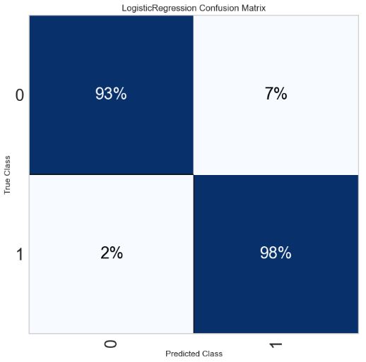
0 0.93 0.93 0.93 1953
1 0.98 0.98 0.98 5892
accuracy 0.96 7845
macro avg 0.95 0.95 0.95 7845
weighted avg 0.96 0.96 0.96 7845
- Plotting the LR normalized confusion matrix using yellowbricks
import yellowbrick

pd.set_option("display.max_columns", 35)

import warnings
warnings.filterwarnings("ignore")
from yellowbrick.classifier import ConfusionMatrix

target_names=['0','1']

fig = plt.figure(figsize=(7,7))
ax = fig.add_subplot(111)

visualizer = ConfusionMatrix(model,
                             classes=target_names,
                             percent=True,
                             cmap="Blues",
                             fontsize=22,
                             ax=ax)

visualizer.fit(X_pca, y_train)

visualizer.score(X_test_pca, y_test)

visualizer.show();
SVC Model
- The same considerations apply to the SVC model
modelsvc = SVC()
modelsvc.fit(X_pca, y_train)
y_pred = modelsvc.predict(X_test_pca)
print(classification_report(y_pred, y_test))
               precision    recall  f1-score   support

           0       0.92      0.95      0.94      1905
           1       0.98      0.97      0.98      5940

    accuracy                           0.97      7845
   macro avg       0.95      0.96      0.96      7845
weighted avg       0.97      0.97      0.97      7845
import yellowbrick

pd.set_option("display.max_columns", 35)

import warnings
warnings.filterwarnings("ignore")
from yellowbrick.classifier import ConfusionMatrix

target_names=['0','1']

fig = plt.figure(figsize=(7,7))
ax = fig.add_subplot(111)

visualizer = ConfusionMatrix(modelsvc,
                             classes=target_names,
                             percent=True,
                             cmap="Blues",
                             fontsize=22,
                             ax=ax)

visualizer.fit(X_pca, y_train)

visualizer.score(X_test_pca, y_test)

visualizer.show();

KNN Model
- Let’s implement the KNeighbors (KNN) Classifier by preparing the input data
df_train=pd.read_csv("dataset_malwares.csv")
X=df_train.drop(['Name','Malware','e_magic',
'SectionMaxEntropy',
'SectionMaxRawsize',
'SectionMaxVirtualsize',
'SectionMinPhysical',
'SectionMinVirtual',
'SectionMinPointerData',
'SectionMainChar'],axis=1)
y=df_train['Malware']
- Splitting the data with test_size=0.4 and training the KNN model
from sklearn.neighbors import KNeighborsClassifier
from sklearn.model_selection import train_test_split
from sklearn.metrics import classification_report, confusion_matrix
import matplotlib.pyplot as plt
import seaborn as sns

def cr(y_test,y_pred):
    ax=sns.heatmap(confusion_matrix(y_pred, y_test), annot=True, fmt="d", cmap=plt.cm.Blues, cbar=False)
    ax.set_xlabel('Predicted labels')
    ax.set_ylabel('True labels')
    print(classification_report(y_test, y_pred, target_names=['Benign', 'Malware']))
from sklearn.model_selection import train_test_split
X_train, X_test, y_train, y_test = train_test_split(X, y, test_size=0.4, random_state=0)
neigh = KNeighborsClassifier(n_neighbors=3)
neigh.fit(X_train, y_train)
y_pred=neigh.predict(X_test)
- Printing the classification report
cr(y_test,y_pred)

               precision    recall  f1-score   support

      Benign       0.97      0.97      0.97      2006
     Malware       0.99      0.99      0.99      5839

    accuracy                           0.99      7845
   macro avg       0.98      0.98      0.98      7845
weighted avg       0.99      0.99      0.99      7845
- Plotting the KNN normalized confusion matrix
import yellowbrick

pd.set_option("display.max_columns", 35)

import warnings
warnings.filterwarnings("ignore")
from yellowbrick.classifier import ConfusionMatrix

target_names=['0','1']

fig = plt.figure(figsize=(7,7))
ax = fig.add_subplot(111)

visualizer = ConfusionMatrix(neigh,
                             classes=target_names,
                             percent=True,
                             cmap="Blues",
                             fontsize=22,
                             ax=ax)

visualizer.fit(X_train, y_train)

visualizer.score(X_test, y_test)

visualizer.show();

Using T-SNE Clustering
- Implementing the t-SNE clustering algorithm
#Using T-SNE
from sklearn.manifold import TSNE
from sklearn.decomposition import PCA
from sklearn.preprocessing import StandardScaler
X_std = StandardScaler().fit_transform(X_train)
pca = PCA(n_components=3)
principalComponents = pca.fit_transform(X_std)
tsne = TSNE(n_components=2, verbose=1, perplexity=80, n_iter=250, learning_rate=100)
tsne_scale_results = tsne.fit_transform(X_std)
tsne_df_scale = pd.DataFrame(tsne_scale_results, columns=['tsne1', 'tsne2'])
plt.figure(figsize = (10,10))
plt.scatter(tsne_df_scale.iloc[:,0],tsne_df_scale.iloc[:,1],alpha=0.25, facecolor='lightslategray')
plt.xlabel('tsne1')
plt.ylabel('tsne2')
plt.show()

[t-SNE] Computing 241 nearest neighbors...
[t-SNE] Indexed 13727 samples in 0.003s...
[t-SNE] Computed neighbors for 13727 samples in 0.575s...
[t-SNE] Computed conditional probabilities for sample 1000 / 13727
[t-SNE] Computed conditional probabilities for sample 2000 / 13727
[t-SNE] Computed conditional probabilities for sample 3000 / 13727
[t-SNE] Computed conditional probabilities for sample 4000 / 13727
[t-SNE] Computed conditional probabilities for sample 5000 / 13727
[t-SNE] Computed conditional probabilities for sample 6000 / 13727
[t-SNE] Computed conditional probabilities for sample 7000 / 13727
[t-SNE] Computed conditional probabilities for sample 8000 / 13727
[t-SNE] Computed conditional probabilities for sample 9000 / 13727
[t-SNE] Computed conditional probabilities for sample 10000 / 13727
[t-SNE] Computed conditional probabilities for sample 11000 / 13727
[t-SNE] Computed conditional probabilities for sample 12000 / 13727
[t-SNE] Computed conditional probabilities for sample 13000 / 13727
[t-SNE] Computed conditional probabilities for sample 13727 / 13727
[t-SNE] Mean sigma: 0.000000
[t-SNE] KL divergence after 250 iterations with early exaggeration: 62.002209

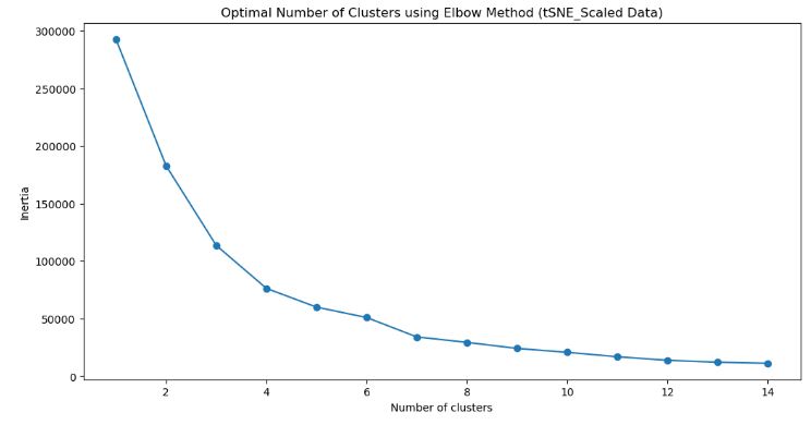
- Let’s check the Optimal Number of Clusters using the Elbow Method (tSNE_Scaled Data)
from sklearn.cluster import KMeans
sse = []
k_list = range(1, 15)
for k in k_list:
    km = KMeans(n_clusters=k)
    km.fit(tsne_df_scale)
    sse.append([k, km.inertia_])

tsne_results_scale = pd.DataFrame({'Cluster': range(1,15), 'SSE': sse})
plt.figure(figsize=(12,6))
plt.plot(pd.DataFrame(sse)[0], pd.DataFrame(sse)[1], marker='o')
plt.title('Optimal Number of Clusters using Elbow Method (tSNE_Scaled Data)')
plt.xlabel('Number of clusters')
plt.ylabel('Inertia')
- Computing the K-Means t-SNE Scaled Silhouette Score
from sklearn.metrics import silhouette_score
kmeans_tsne_scale = KMeans(n_clusters=2, n_init=100, max_iter=400, init='k-means++', random_state=42).fit(tsne_df_scale)
print('KMeans tSNE Scaled Silhouette Score: {}'.format(silhouette_score(tsne_df_scale, kmeans_tsne_scale.labels_, metric='euclidean')))
labels_tsne_scale = kmeans_tsne_scale.labels_
clusters_tsne_scale = pd.concat([tsne_df_scale, pd.DataFrame({'tsne_clusters':labels_tsne_scale})], axis=1)
KMeans tSNE Scaled Silhouette Score: 0.38039013743400574
- Plotting the Cluster Visual t-SNE Scaled Data
plt.scatter(clusters_tsne_scale.iloc[:,0],clusters_tsne_scale.iloc[:,1],c=labels_tsne_scale)
plt.xlabel('tsne1')
plt.ylabel('tsne2')
plt.colorbar()
plt.show()

- One can see a decision boundary that separates t-SNE scaled data points belonging to different binary class labels (0 and 1).
Decision Tree (DT) Tuning
- Let’s optimize the Decision Tree (DT) Classifier by comparing validation curves and related classification metrics for an arbitrary DT model and a set of hyperparameters.
- Preparing the input data, running the DT classifier with criterion = “entropy” and variable Maximum Tree Depth (MTD<32), while collecting statistics such as accuracy and log-loss
# Reading the input data

import pandas as pd
import numpy as np

data = pd.read_csv("dataset_malwares.csv")

#train/test splitting

from sklearn.model_selection import train_test_split

rs=42

X_train, X_val, y_train, y_val = train_test_split(data.drop(["Name", "Malware", "CheckSum"], axis = 1),
                                                  data["Malware"], test_size = 0.3, random_state = rs)
stat_range = range(30)

#Running DT and collecting statistics

def collect_statistics(create_classifier, list_initializers, Xtrain = X_train, ytrain = y_train, Xval = X_val, yval = y_val):

    stats = [ [] for l in range(len(list_initializers)) ]

    for i in stat_range:
        model = create_classifier(i)
        model.fit(Xtrain, ytrain)

        y = model.predict(Xval)
        p = model.predict_proba(Xval)
        p0 = p[yval == 0, 0]
        p1 = p[yval == 1, 1]

        for l in zip(stats, list_initializers):
            l[0].append(l[1](y, p, p0, p1))

    return tuple(stats)


from sklearn.tree import DecisionTreeClassifier
from sklearn.metrics import accuracy_score
from sklearn.metrics import log_loss
from sklearn.metrics import recall_score
from sklearn.metrics import precision_score
from sklearn.metrics import f1_score
from math import ceil

import matplotlib.pyplot as plt
%matplotlib inline

color1 = "#333399"
color2 = "#FF5733"
color3 = "#008264"
lss = { "linewidth" : 2 }
lss2 = { "linewidth" : 2, "linestyle" : (0, (7, 2)) }
lss3 = { "linewidth" : 2, "linestyle" : "--" }

def set_figure_size(h, w):
    plt.rcParams["figure.figsize"] = (ceil((13.0 * w)/2.0), 5 * h)

cart_depth_lim = lambda x: DecisionTreeClassifier(criterion = "entropy", max_depth = x + 2, random_state = rs)
cart_depth_lim_depths = lambda x: [ i + 2 for i in x ]
cart_depth_lim_depths_name = "Maximum Tree Depth"

atrs, lsrs = collect_statistics(cart_depth_lim, [ lambda y, p, p0, p1: accuracy_score(y_val, y),
                                                  lambda y, p, p0, p1: log_loss(y_val, p) ] )

plt.rcParams.update({'font.size': 14})

set_figure_size(1, 2)

plt.subplot(1, 2, 1)
plt.plot(cart_depth_lim_depths(stat_range), atrs, color1, **lss)
plt.tight_layout()
plt.title("Accuracy of Decision Tree Classifier")
plt.xlabel(cart_depth_lim_depths_name)
plt.ylabel("Accuracy")
plt.grid(True)

plt.subplot(1, 2, 2)
plt.plot(cart_depth_lim_depths(stat_range), lsrs, color1, **lss)
plt.tight_layout()
plt.title("Cross-entropy Loss of Decision Tree Classifier")
plt.xlabel(cart_depth_lim_depths_name)
plt.ylabel("Log-loss")
plt.grid(True)
plt.show()

- Applying hyperparameter optimization using GridSearchCV
from sklearn.model_selection import GridSearchCV

parameters = { "max_depth" : cart_depth_lim_depths(stat_range) }
clf = GridSearchCV(DecisionTreeClassifier(criterion = "entropy", random_state = rs),
                   parameters, cv = 5, scoring = 'recall')
clf.fit(X_train, y_train)
best_max_depth = clf.best_params_['max_depth']
print("Best value of max_depth:", best_max_depth)

model_best_recall = DecisionTreeClassifier(criterion = "entropy", random_state = rs,
                                           max_depth = best_max_depth)
model_best_recall.fit(X_train, y_train)
yp = model_best_recall.predict(X_val)
print("Recall:", recall_score(y_val, yp))
print("Precision:", precision_score(y_val, yp))
print("Accuracy:", accuracy_score(y_val, yp))

Best value of max_depth: 6
Recall: 0.9988594890510949
Precision: 0.982499439084586
Accuracy: 0.9858939496940856
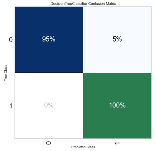
- Computing and plotting the normalized confusion matrix
from sklearn.metrics import confusion_matrix
tn, fp, fn, tp = confusion_matrix(y_val, model_best_recall.predict(X_val)).ravel()
print("Number of false positives:", fp)
print("Number of false negatives:", fn)
Number of false positives: 78
Number of false negatives: 5
import yellowbrick

pd.set_option("display.max_columns", 35)

import warnings
warnings.filterwarnings("ignore")
from yellowbrick.classifier import ConfusionMatrix

target_names=['0','1']

fig = plt.figure(figsize=(7,7))
ax = fig.add_subplot(111)

visualizer = ConfusionMatrix(model_best_recall,
                             classes=target_names,
                             percent=True,
                             cmap="Blues",
                             fontsize=22,
                             ax=ax)

visualizer.fit(X_train, y_train)

visualizer.score(X_val, y_val)

visualizer.show();
- Running the optimized/balanced Decision Tree Classifier with max_depth = best_max_depth, class_weight = “balanced”
from sklearn.tree import export_graphviz
model_best_recall_bal = DecisionTreeClassifier(criterion = "entropy", random_state = rs,
                                            max_depth = best_max_depth, class_weight = "balanced")
model_best_recall_bal.fit(X_train, y_train)
dot_data = export_graphviz(model_best_recall_bal,
                           max_depth = 1,
                           out_file = None, feature_names = list(X_train.columns.values),
                           class_names=["Benign", "Malware"],  filled = True, rounded = True,
                           special_characters = True)
- Computing and plotting Precision and Recall of the Decision Tree Classifier vs Maximum Tree Depth
cart_depth_lim_bal = lambda i: DecisionTreeClassifier(criterion = "entropy", class_weight = "balanced",
                                                      max_depth = i + 2, random_state = rs)

recs_b, precs_b = collect_statistics(cart_depth_lim_bal, [ lambda y, p, p0, p1: recall_score(y_val, y),
                                                           lambda y, p, p0, p1: precision_score(y_val, y) ] )

#import matplotlib
#plt.rcParams["figure.figsize"] = (13,5)
plt.figure(figsize=(10,5))
plt.rcParams.update({'font.size': 22})
#matplotlib.rcParams.update({'font.size': 14})

set_figure_size(1, 2)

plt.subplot(1, 2, 1)
plt.plot(cart_depth_lim_depths(stat_range), precs_b, color1, **lss)
plt.tight_layout()
plt.title("Precision of Balanced Decision Tree Classifier")
plt.xlabel(cart_depth_lim_depths_name)
plt.ylabel("Precision")
plt.grid(True)

plt.subplot(1, 2, 2)
plt.plot(cart_depth_lim_depths(stat_range), recs_b, color1, **lss)
plt.tight_layout()
plt.title("Recall of Balanced Decision Tree Classifier")
plt.xlabel(cart_depth_lim_depths_name)
plt.ylabel("Recall")
plt.grid(True)
plt.show()
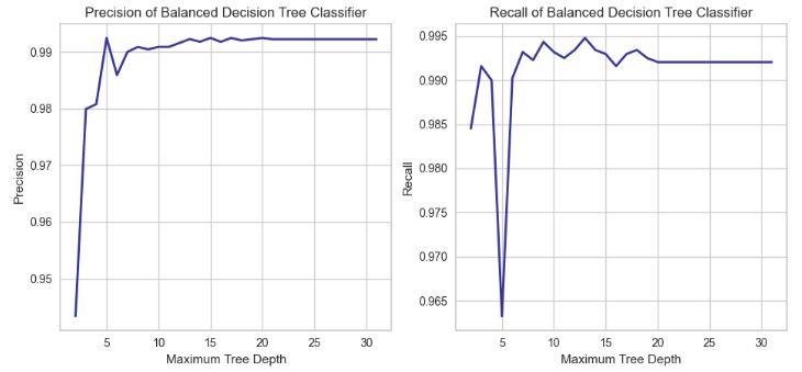
- The recall score no longer displays a pronounced decrease trend as the limit on the tree depth grows.
- For our dataset with unbalanced labels, we need to use
balanced_accuracy()instead ofaccuracy(), provided all the classes are treated on equal footing.
from sklearn.metrics import balanced_accuracy_score

#comma after batrs "unpacks" the tuple returned by collect_statistics()
batrs, = collect_statistics(cart_depth_lim, [ lambda y, p, p0, p1: balanced_accuracy_score(y_val, y) ] )

set_figure_size(1, 1)

plt.plot(cart_depth_lim_depths(stat_range), atrs, color1, cart_depth_lim_depths(stat_range), batrs, color2, **lss)
plt.tight_layout()
plt.title("Accuracy of Decision Tree Classifier")
plt.xlabel(cart_depth_lim_depths_name)
plt.ylabel("Accuracy")
plt.legend(["Accuracy", "Balanced Accuracy"], loc = "center right")
plt.grid(True)

- Plotting the F1 score-based curve for the regular DT and the log-loss curve for the balanced DT
#comma after batrs "unpacks" the tuple returned by collect_statistics()
f1s, = collect_statistics(cart_depth_lim, [ lambda y, p, p0, p1: f1_score(y_val, y) ] )

cart_depth_lim_bal = lambda i: DecisionTreeClassifier(criterion = "entropy", class_weight = "balanced",
                                                      max_depth = i + 2, random_state = rs)
atrs_b, = collect_statistics(cart_depth_lim_bal, [ lambda y, p, p0, p1: log_loss(y_val, p) ] )

plt.figure(figsize=(10,5))
plt.rcParams.update({'font.size': 22})

set_figure_size(1, 2)

plt.subplot(1, 2, 1)
plt.plot(cart_depth_lim_depths(stat_range), f1s, color1, **lss)
plt.tight_layout()
plt.title("F1 Score of Decision Tree Classifier")
plt.xlabel(cart_depth_lim_depths_name)
plt.ylabel("F1")
plt.grid(True)

plt.subplot(1, 2, 2)
plt.plot(cart_depth_lim_depths(stat_range), atrs_b, color1, **lss)
plt.tight_layout()
plt.title("Log-Loss of Balanced Decision Tree Classifier")
plt.xlabel(cart_depth_lim_depths_name)
plt.ylabel("Accuracy")
plt.grid(True)

plt.show()

- Plotting the normalized confusion matrix for the balanced Decision Tree Classifier
import yellowbrick

pd.set_option("display.max_columns", 35)

import warnings
warnings.filterwarnings("ignore")
from yellowbrick.classifier import ConfusionMatrix

target_names=['0','1']

fig = plt.figure(figsize=(7,7))
ax = fig.add_subplot(111)

visualizer = ConfusionMatrix(model_best_recall_bal,
                             classes=target_names,
                             percent=True,
                             cmap="Blues",
                             fontsize=22,
                             ax=ax)

visualizer.fit(X_train, y_train)

visualizer.score(X_val, y_val)

visualizer.show();

XGBoost Classifier
- Applying the XGBoost Classifier to the training data
import xgboost as xgb
modelxgb = xgb.XGBClassifier()
modelxgb.fit(X_train, y_train)


 XGBClassifier:
XGBClassifier(base_score=0.5, booster='gbtree', callbacks=None,
              colsample_bylevel=1, colsample_bynode=1, colsample_bytree=1,
              early_stopping_rounds=None, enable_categorical=False,
              eval_metric=None, gamma=0, gpu_id=-1, grow_policy='depthwise',
              importance_type=None, interaction_constraints='',
              learning_rate=0.300000012, max_bin=256, max_cat_to_onehot=4,
              max_delta_step=0, max_depth=6, max_leaves=0, min_child_weight=1,
              missing=nan, monotone_constraints='()', n_estimators=100,
              n_jobs=0, num_parallel_tree=1, predictor='auto', random_state=0,
              reg_alpha=0, reg_lambda=1, ...)
- Making predictions and creating the classification report
predictions = modelxgb.predict(X_val)
X = data.drop(['Name', 'Malware'], axis = 1)
y = data['Malware']
from sklearn.model_selection import train_test_split
X_train, X_test, y_train, y_test = train_test_split(X, y, test_size=0.4, random_state=0)
modelxgb.fit(X_train, y_train)
predictions = modelxgb.predict(X_test)
#Calculating accuracy
accuracy = accuracy_score(y_test, predictions)

target_names=['0','1']

print("Accuracy:", accuracy)
print("\nClassification Report:")
print(classification_report(y_test, predictions, target_names=target_names))
Accuracy: 0.9936265137029955

Classification Report:
              precision    recall  f1-score   support

           0       0.99      0.98      0.99      2006
           1       0.99      1.00      1.00      5839

    accuracy                           0.99      7845
   macro avg       0.99      0.99      0.99      7845
weighted avg       0.99      0.99      0.99      7845
- Calculating and plotting the normalized confusion matrix
import yellowbrick
from sklearn.metrics import classification_report

pd.set_option("display.max_columns", 35)

import warnings
warnings.filterwarnings("ignore")
from yellowbrick.classifier import ConfusionMatrix

target_names=['0','1']

fig = plt.figure(figsize=(7,7))
ax = fig.add_subplot(111)

visualizer = ConfusionMatrix(modelxgb,
                             classes=target_names,
                             percent=True,
                             cmap="Blues",
                             fontsize=22,
                             ax=ax)

visualizer.fit(X_train, y_train)

visualizer.score(X_test, y_test)

visualizer.show();

Other Classifiers
- Importing other SciKit-Learn classifiers
import pandas as pd
import numpy as np
import matplotlib
import matplotlib.pyplot as plt
import seaborn as sns
from sklearn.preprocessing import LabelEncoder
from statsmodels.stats.outliers_influence import variance_inflation_factor
from sklearn.model_selection import train_test_split
from sklearn.preprocessing import StandardScaler
from sklearn.linear_model import LogisticRegression
from sklearn.svm import SVC
from sklearn.neighbors import KNeighborsClassifier
from sklearn.naive_bayes import GaussianNB
from sklearn.tree import DecisionTreeClassifier
from sklearn.ensemble import RandomForestClassifier
from sklearn.metrics import confusion_matrix, accuracy_score
from sklearn.metrics import f1_score, precision_score, recall_score, fbeta_score
from sklearn.model_selection import cross_val_score
from sklearn.model_selection import GridSearchCV
from sklearn.model_selection import ShuffleSplit
from sklearn.model_selection import KFold
from sklearn import feature_selection
from sklearn import model_selection
from sklearn.metrics import auc, roc_auc_score, roc_curve
%matplotlib inline
#Other classifiers
from sklearn.tree import ExtraTreeClassifier
from sklearn.tree import DecisionTreeClassifier
from sklearn.svm import OneClassSVM
from sklearn.neural_network import MLPClassifier
from sklearn.neighbors import RadiusNeighborsClassifier
from sklearn.neighbors import KNeighborsClassifier
from sklearn.multioutput import ClassifierChain
from sklearn.multioutput import MultiOutputClassifier
from sklearn.multiclass import OutputCodeClassifier
from sklearn.multiclass import OneVsOneClassifier
from sklearn.multiclass import OneVsRestClassifier
from sklearn.linear_model import SGDClassifier
from sklearn.linear_model import RidgeClassifierCV
from sklearn.linear_model import RidgeClassifier
from sklearn.linear_model import PassiveAggressiveClassifier
from sklearn.gaussian_process import GaussianProcessClassifier
from sklearn.ensemble import VotingClassifier
from sklearn.ensemble import AdaBoostClassifier
from sklearn.ensemble import GradientBoostingClassifier
from sklearn.ensemble import BaggingClassifier
from sklearn.ensemble import ExtraTreesClassifier
from sklearn.ensemble import RandomForestClassifier
from sklearn.naive_bayes import BernoulliNB
from sklearn.calibration import CalibratedClassifierCV
from sklearn.naive_bayes import GaussianNB
from sklearn.semi_supervised import LabelPropagation
from sklearn.semi_supervised import LabelSpreading
from sklearn.discriminant_analysis import LinearDiscriminantAnalysis
from sklearn.svm import LinearSVC
from sklearn.linear_model import LogisticRegression
from sklearn.linear_model import LogisticRegressionCV
from sklearn.naive_bayes import MultinomialNB
from sklearn.neighbors import NearestCentroid
from sklearn.svm import NuSVC
from sklearn.linear_model import Perceptron
from sklearn.discriminant_analysis import QuadraticDiscriminantAnalysis
from sklearn.svm import SVC
from sklearn.mixture import GaussianMixture
from sklearn.model_selection import cross_val_score
- Running the MLP Classifier
classifier = MLPClassifier()
classifier.fit(X_train, y_train)
y_pred = classifier.predict(X_test)
accuracies = cross_val_score(estimator =classifier,X = X_train, y = y_train, cv = 10)
print("MLP Classifier Accuracy: %0.2f (+/- %0.2f)"  % (accuracies.mean(),
accuracies.std()*2))
MLP Classifier Accuracy: 0.85 (+/- 0.15)
- Running the GaussianNB classifier
classifier = GaussianNB()
classifier.fit(X_train, y_train)
y_pred = classifier.predict(X_test)
accuracies = cross_val_score(estimator =classifier,X = X_train, y = y_train, cv = 10)
print("GNB Classifier Accuracy: %0.2f (+/- %0.2f)"  % (accuracies.mean(),
accuracies.std()*2))
GNB Classifier Accuracy: 0.32 (+/- 0.01)
- Running the HistGradientBoosting (HGB) Classifier
from sklearn.ensemble import HistGradientBoostingClassifier
classifier = HistGradientBoostingClassifier()
classifier.fit(X_train, y_train)
y_pred = classifier.predict(X_test)
accuracies = cross_val_score(estimator =classifier,X = X_train, y = y_train, cv = 10)
print("HGB Classifier Accuracy: %0.2f (+/- %0.2f)"  % (accuracies.mean(),
accuracies.std()*2))
HGB Classifier Accuracy: 0.99 (+/- 0.00)
- Plotting the HGB classification report
#Calculating accuracy
accuracy = accuracy_score(y_test, y_pred)

target_names=['0','1']

print("Accuracy:", accuracy)
print("\nClassification Report:")
print(classification_report(y_test, y_pred, target_names=target_names))
Accuracy: 0.9932441045251753

Classification Report:
              precision    recall  f1-score   support

           0       0.99      0.98      0.99      2006
           1       0.99      1.00      1.00      5839

    accuracy                           0.99      7845
   macro avg       0.99      0.99      0.99      7845
weighted avg       0.99      0.99      0.99      7845
Summary
- Malware detection is an important security topic with strong associations with legal, reputational, and economic concerns of organizations worldwide.
- The present project has examined the potential of applying PCA, T-SNE and optimized supervised Machine Learning (ML) binary classification algorithms to malware detection & interpretation.
- A collected benchmark dataset of authentic malware samples has been analyzed to evaluate ML techniques in terms of commonly employed performance metrics.
- An F1 score of 99%, a precision of 99%, a recall of 99% and an accuracy of 99% were all achieved for the KNN and optimized Decision Tree models.
- Other high-performing ML models are Logistic Regression, SVC, XGBoost, and HistGradientBoosting.
- It has been shown that the t-SNE visualization can separate benign and malicious data from PE files. We have observed a distinct decision boundary that delineates the boundaries of 2 classes with a negligible contamination. It is clear that 2D t-SNE is able to recover well-separated binary clusters of malware samples.
- Results have confirmed that cybersecurity experts can boost malware detection rates using ML algorithms, lower false positives and accelerate malware detection.
- Our next project will focus on applying deep reinforcement learning to tell the difference between harmful and harmless files.
Explore More
- Effective AI-Powered Malware Detection & Interpretation – 1. H2O AutoML
- Robust Fake News Detection: NLP Algorithms for Deep Learning and Supervised ML in Python
- Comparison of 20 ML NLP Algorithms for SMS Spam-Ham Binary Classification
- Bank Note Authentication – Classification
- Improved Multiple-Model ML/DL Credit Card Fraud Detection: F1=88% & ROC=91%
- Data-Driven ML Credit Card Fraud Detection


One-Time
Monthly
Yearly
Make a one-time donation
Make a monthly donation
Make a yearly donation
Choose an amount
€5.00
€15.00
€100.00
€5.00
€15.00
€100.00
€5.00
€15.00
€100.00
Or enter a custom amount
€
Your contribution is appreciated.
Your contribution is appreciated.
Your contribution is appreciated.
DonateDonate monthlyDonate yearly
Leave a comment