Anatomy of the Robust 1D Kalman Filter

The Kalman Filter (KF) is a robust tool for creating the optimal solution to many tracking, navigation, and data prediction tasks.
This article outlines a simplified implementation of KF with commonly used Python commands.
The main purpose of proposing a tutorial like this is to allow readers clearly understand KF without much knowledge in numerical optimization methods and digital signal processing.
KF is an optimal state estimator under the assumption of linearity and Gaussian noise. It considers that all measured data have a certain error compared to the actual states. By comparing the next observed state and the predicted state, the predicted model can be iteratively updated.
KF minimizes posterior state estimation, which is equivalent to saying it minimizes mean-square error estimator.
The most important concepts are that KF are discrete in time and recursive. In addition, KF predict the future by deriving an adjusted estimate of a state from both prediction and measurements.

The basic 1D Kalman filter algorithm is implemented as follows:
1. Input the measurement vector z as a function of states and
2. Input the RMS deviation of sensor data noise R;
3. Define the initial state x(k)=0 and P(k)=1, where k=0;
4. Set k=k+1 and define the state prediction x*(k)=x(k-1) and the prior error covariance P*(k)=P(k-1);
5. Compute the Kalman gain K(k) = P*(k)/(P*(k)+R)
6. Update the error covariance P(k) = {1-K(k)} x P*(k)
7. Correct the state x(k) = x*(k) + K(k) x {z(k)-x*(k)}

Let’s look at several simple illustrative examples of using KF aimed at building intuition and experience, not formal proofs.

Table of Contents

A Simple 1D Voltage Reading
Linear True State & Random Noise
1D Object Tracking
1D State Space Models and Kalman Filtering
KO Log Returns
Minimal 1D Kalman Filter
1D Kalman Smoothing
1D Kalman Time-Series Prediction
Summary
References

A Simple 1D Voltage Reading

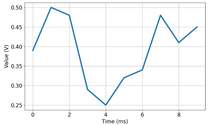
Following the quick guide, let’s consider a scalar constant voltage reading a V with the standard deviation of noisy readings of R=0.1 V:

import matplotlib.pyplot as plt
ys = [0.39,0.50,0.48,0.29,0.25,0.32,0.34,0.48,0.41,0.45]
xs = [x for x in range(len(ys))]

plt.figure(figsize=(10,6))
plt.rcParams.update({'font.size': 16})
plt.plot(xs, ys,lw=4)
plt.xlabel('Time (ms)') 
plt.ylabel('Value (V)')
plt.grid()
plt.show()

Noisy measurement of a scalar constant voltage reading (V).

Defining the initial state parameters

pvec = [1.0,1.0,1.0,1.0,1.0,1.0,1.0,1.0,1.0,1.0]
yk = [0.0,0.0,0.0,0.0,0.0,0.0,0.0,0.0,0.0,0.0]
kvec=[0.0,0.0,0.0,0.0,0.0,0.0,0.0,0.0,0.0,0.0]
rpar=0.1

KF update with k=0

kvec[0]=pvec[0]/(pvec[0]+rpar)
print(kvec[0])
0.9090909090909091
pvec[0]=(1.0-kvec[0])*pvec[0]
print(pvec[0])
0.09090909090909094
yk[0]=yk[0]+kvec[0]*(ys[0]-yk[0])
print(yk[0])
0.35454545454545455

KF update with k=1

kvec[1]=pvec[0]/(pvec[0]+rpar)
print(kvec[1])
0.4761904761904763
pvec[1]=(1.0-kvec[1])*pvec[0]
print(pvec[1])
0.04761904761904763
yk[1]=yk[0]+kvec[1]*(ys[1]-yk[0])
print(yk[1])
0.42380952380952386

KF update with k=2

kvec[2]=pvec[1]/(pvec[1]+rpar)
print(kvec[2])
0.3225806451612903
pvec[2]=(1.0-kvec[2])*pvec[1]
print(pvec[2])
0.032258064516129045
yk[2]=yk[1]+kvec[2]*(ys[2]-yk[1])
print(yk[2])
0.44193548387096776

KF update with k=3

kvec[3]=pvec[2]/(pvec[2]+rpar)
print(kvec[3])
0.24390243902439032
pvec[3]=(1.0-kvec[3])*pvec[2]
print(pvec[3])
0.024390243902439032
yk[3]=yk[2]+kvec[3]*(ys[3]-yk[2])
print(yk[3])
0.40487804878048783

KF update with k=4

kvec[4]=pvec[3]/(pvec[3]+rpar)
print(kvec[4])
0.19607843137254907
pvec[4]=(1.0-kvec[4])*pvec[3]
print(pvec[4])
0.019607843137254905
yk[4]=yk[3]+kvec[4]*(ys[4]-yk[3])
print(yk[4])
0.37450980392156863

KF update with k=5

k=5
kvec[k]=pvec[k-1]/(pvec[k-1]+rpar)
print(kvec[k])
0.1639344262295082
pvec[k]=(1.0-kvec[k])*pvec[k-1]
print(pvec[k])
0.016393442622950824
yk[k]=yk[k-1]+kvec[k]*(ys[k]-yk[k-1])
print(yk[k])
0.3655737704918033

KF update with k=6

k=6
kvec[k]=pvec[k-1]/(pvec[k-1]+rpar)
print(kvec[k])
0.14084507042253525
pvec[k]=(1.0-kvec[k])*pvec[k-1]
print(pvec[k])
0.014084507042253525
yk[k]=yk[k-1]+kvec[k]*(ys[k]-yk[k-1])
print(yk[k])
0.3619718309859155

KF update with k=7

k=7
kvec[k]=pvec[k-1]/(pvec[k-1]+rpar)
print(kvec[k])
0.12345679012345681
pvec[k]=(1.0-kvec[k])*pvec[k-1]
print(pvec[k])
0.012345679012345682
yk[k]=yk[k-1]+kvec[k]*(ys[k]-yk[k-1])
print(yk[k])
0.3765432098765432

KF update with k=8

k=8
kvec[k]=pvec[k-1]/(pvec[k-1]+rpar)
print(kvec[k])
0.10989010989010992
pvec[k]=(1.0-kvec[k])*pvec[k-1]
print(pvec[k])
0.010989010989010992
yk[k]=yk[k-1]+kvec[k]*(ys[k]-yk[k-1])
print(yk[k])
0.3802197802197802

KF update with k=9

k=9
kvec[k]=pvec[k-1]/(pvec[k-1]+rpar)
print(kvec[k])
0.09900990099009903
pvec[k]=(1.0-kvec[k])*pvec[k-1]
print(pvec[k])
0.009900990099009903
yk[k]=yk[k-1]+kvec[k]*(ys[k]-yk[k-1])
print(yk[k])
0.38712871287128714

Plotting observed values vs KF (predicted/corrected) updates

plt.figure(figsize=(10,6))
plt.rcParams.update({'font.size': 16})

plt.plot(xs, ys,label='Observed',lw=4)
plt.plot(xs, yk,label='Kalman Filter',lw=4)
ax.legend(handles=[line1, line2])
plt.xlabel('Time (ms)') 
plt.ylabel('Value (V)')
plt.legend(loc="lower right")
plt.grid()
plt.show()

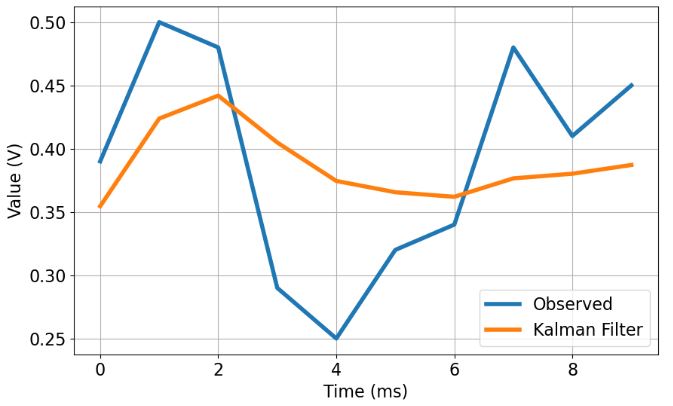
Observed values vs KF (predicted/corrected) updates

This plot shows that KF converges to the true voltage value over 8 iterations

import statistics
ykmean=statistics.mean(yk)
print(ykmean)
0.3871115619373332

The KF prediction error is within the confidence interval

ykstd=statistics.stdev(yk)
print(ykstd)
0.028171057014034436

Indeed, we can see that

ysmean=statistics.mean(ys)
print(ysmean)
0.391
ysstd=statistics.stdev(ys)
print(ysstd)
0.08774331250237187

Linear True State & Random Noise

Let’s consider a 1D linear true (simulated) state and measurements with random noise. The KF is expressed in terms of the process and measurement noise covariances Q and R, respectively. Our goal is to examine the suitability of the basic KF algorithm for these measurements:

import numpy as np
import matplotlib.pyplot as plt
from matplotlib.animation import FuncAnimation, PillowWriter

#Animation to plot incrementally for each time step
def animate(i):
    #Clear previous plot
    ax.clear()

    #Plot to desired time step

    plt.plot(x[:i+1], true_states[0][:i+1], label='True State', markersize=10, color='blue')
    plt.plot(x[:i+1], measurements[:i+1], 'rx', label='Measurements', markersize=10, color='red')
    plt.plot(x[:i+1], filtered_states[0][:i+1], label='Filtered State', color='green')
    plt.title('Kalman Filter Position Q=1.0 R=1.0')
    plt.xlabel('Time Steps')
    plt.ylabel('Position')
    plt.legend()


# Kalman filter parameters
dt = 1.0  # Time step
A = np.array([[1, dt], [0, 1]])  # State transition matrix
H = np.array([[1, 0]])  # Measurement matrix
Q = 1.0* np.eye(2)  # Process noise covariance
R = 0.1  # Measurement noise covariance

# Initial state estimate
x_hat = np.array([[0], [0]])

# Initial covariance estimate
P = np.eye(2)

# Number of time steps
num_steps = 50
x = np.arange(num_steps)

# True state (simulated)
true_states = np.linspace(0, 2 * np.pi, num_steps)
true_positions = np.cos(true_states)
true_states = np.vstack((true_states, true_positions))

# Measurements with noise
measurements = true_states[0, :] + np.sqrt(R) * np.random.randn(num_steps)

# Kalman filter loop
filtered_states = np.zeros((2, num_steps))

for k in range(num_steps):
    # Prediction step
    x_hat_minus = A.dot(x_hat)
    P_minus = A.dot(P).dot(A.T) + Q

    # Update step
    K = P_minus.dot(H.T).dot(np.linalg.inv(H.dot(P_minus).dot(H.T) + R))
    x_hat = x_hat_minus + K.dot(measurements[k] - H.dot(x_hat_minus))
    P = (np.eye(2) - K.dot(H)).dot(P_minus)

    filtered_states[:, k] = x_hat.flatten()


# Create a figure and axis
fig, ax = plt.subplots()

#Save animation as gif
animation = FuncAnimation(fig, animate, frames=num_steps, interval=400, repeat=False)
animation.save('kalman_filter_animation.gif', writer='pillow', fps=5)
plt.show()

Plotting the KF position vs time steps for different values of noise covariances

The Kalman filter position vs time steps for Q=10 and R=0.01

The Kalman filter position vs time steps for Q=0.01 and R=0.01

The Kalman filter position vs time steps for Q=10 and R=1.0

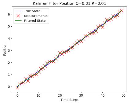
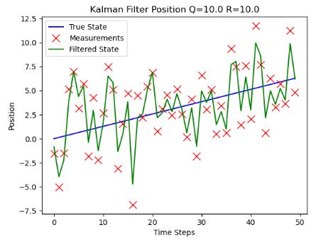
As expected, robustness of KF with respect to both noise covariances is observed.

1D Object Tracking

Let’s apply the KF in tracking an object in a 1-D direction using Python. In doing so, we introduce the following class

class KalmanFilter(object):
    def __init__(self, dt, u, std_acc, std_meas):
        self.dt = dt
        self.u = u
        self.std_acc = std_acc
        self.A = np.matrix([[1, self.dt],
                            [0, 1]])
        self.B = np.matrix([[(self.dt**2)/2], [self.dt]]) 
        self.H = np.matrix([[1,0]])
        self.Q = np.matrix([[(self.dt**4)/4, (self.dt**3)/2],
                            [(self.dt**3)/2, self.dt**2]]) * self.std_acc**2
        self.R = std_meas**2
        self.P = np.eye(self.A.shape[1])
        self.x = np.matrix([[0],[0]])
    def predict(self):
        # Ref :Eq.(9) and Eq.(10)
        # Update time state
        self.x = np.dot(self.A, self.x) + np.dot(self.B, self.u)
        # Calculate error covariance
        # P= A*P*A' + Q
        self.P = np.dot(np.dot(self.A, self.P), self.A.T) + self.Q
        return self.x
    def update(self, z):
        # Ref :Eq.(11) , Eq.(11) and Eq.(13)
        # S = H*P*H'+R
        S = np.dot(self.H, np.dot(self.P, self.H.T)) + self.R
        # Calculate the Kalman Gain
        # K = P * H'* inv(H*P*H'+R)
        K = np.dot(np.dot(self.P, self.H.T), np.linalg.inv(S))  # Eq.(11)
        self.x = np.round(self.x + np.dot(K, (z - np.dot(self.H, self.x))))  # Eq.(12)
        I = np.eye(self.H.shape[1])
        self.P = (I - (K * self.H)) * self.P  # Eq.(13)

The main function defines a model track and creates the KF object by plotting the result of KF predictions vs measurements

def main():
    dt = 0.1
    t = np.arange(0, 100, dt)
    # Define a model track
    real_track = 0.1*((t**2) - t)
    u= 2
    std_acc = 0.25     # we assume that the standard deviation of the acceleration is 0.25 (m/s^2)
    std_meas = 1.2    # and standard deviation of the measurement is 1.2 (m)
    # create KalmanFilter object
    kf = KalmanFilter(dt, u, std_acc, std_meas)
    predictions = []
    measurements = []
    for x in real_track:
        # Mesurement
        z = kf.H * x + np.random.normal(0, 50)
        measurements.append(z.item(0))
        predictions.append(kf.predict()[0])
        kf.update(z.item(0))
    fig = plt.figure()
    fig.suptitle('Example of Kalman filter for tracking a moving object in 1-D', fontsize=20)
    plt.plot(t, measurements, label='Measurements', color='b',linewidth=0.5)
    plt.plot(t, np.array(real_track), label='Real Track', color='y', linewidth=1.5)
    plt.plot(t, np.squeeze(predictions), label='Kalman Filter Prediction', color='r', linewidth=1.5)
    plt.xlabel('Time (s)', fontsize=20)
    plt.ylabel('Position (m)', fontsize=20)
    plt.legend()
    plt.show()

Plotting the KF predictions vs measurements and real track

if __name__ == '__main__':
    main()

Example of Kalman filter for tracking a moving object in 1-D

The above figure shows the simulation performance of 1D KF for the above case. We can see that it handles noisy measurements pretty well. Specifically, KF can help handle random noise or outliers by reducing the impact of individual data points.
Read more about the aforementioned KF implementation here.

1D State Space Models and Kalman Filtering

To demonstrate the implementation of 1D state space models and KF, let’s generate some synthetic data with Gaussian noise:

import numpy as np
import matplotlib.pyplot as plt
np.random.seed(0)

# Define the number of time steps
T = 200

# Define the state transition matrix
F = np.array([[1]])

# Define the observation matrix
H = np.array([[1]])

# Define the process noise covariance
Q = np.array([[0.05]])

# Define the observation noise covariance
R = np.array([[1]])

# Define the initial state
x0 = np.array([0])

# Generate the true state and observations
x_true = np.zeros((T, 1))
y = np.zeros(T)

x_true[0] = x0
y[0] = H @ np.asarray(x_true[0]) + np.random.multivariate_normal(np.zeros((1,)), R)

for t in range(1, T):
    x_true[t] = F @ x_true[t-1] + np.random.multivariate_normal(np.zeros((1,)), Q)
    y[t] = H @ np.asarray(x_true[t]) + np.random.multivariate_normal(np.zeros((1,)), R)

# Initialize the state estimate and covariance
x_hat = np.zeros((T, 1))
P = np.zeros((T, 1, 1))

x_hat[0] = x0
P[0] = Q

# Run the Kalman filter
for t in range(1, T):
    # Prediction step
    x_hat[t] = F @ x_hat[t-1]
    P[t] = F @ P[t-1] @ F.T + Q

    # Update step
    K = P[t] @ H.T @ np.linalg.inv(H @ P[t] @ H.T + R)
    x_hat[t] = x_hat[t] + K @ (y[t] - H @ x_hat[t])
    P[t] = (np.eye(1) - K @ H) @ P[t]

Plotting the true states, observations and estimated states

# Plot the true states, observations and estimated states
plt.figure(figsize=(10, 6))
plt.rcParams.update({'font.size': 18})
plt.plot(range(T), x_true, label='True States',lw=4,color='red')
plt.plot(range(T), y, label='Observations',lw=4,color='orange')
plt.plot(range(T), x_hat, label='Estimated States',lw=4,color='green')
plt.xlabel('Time')
plt.ylabel('State')
plt.legend()
plt.show()

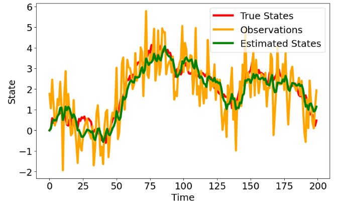
True states, observations and estimated states for synthetic data with Gaussian noise.

This test demonstrates that state space models and KF are powerful tools for modeling and estimating the underlying states of a system based on noisy observations.

KO Log Returns

Let’s apply the above KF technique to the real KO stock price data:

import yfinance as yf

# Download stock price data
data = yf.download('KO', start='2023-01-01', end='2024-01-26')
[*********************100%%**********************]  1 of 1 completed

Computing log returns and removing missing values

# Compute log returns
data['Log Returns'] = np.log(data['Close']).diff()

# Remove missing values
data = data.dropna()

Defining input KF parameters, initializing and running KF

# Define the state transition matrix
F = np.array([[1]])

# Define the observation matrix
H = np.array([[1]])

# Define the process noise covariance
Q = np.array([[0.1]])

# Define the observation noise covariance
R = np.array([[0.01]])

# Define the initial state
x0 = np.array([0])

# Define the number of time steps
T = len(data)

# Generate the observations
y = data['Log Returns'].values.reshape(-1, 1)

# Initialize the state estimate and covariance
x_hat = np.zeros((T, 1))
P = np.zeros((T, 1, 1))

x_hat[0] = x0
P[0] = Q

# Run the Kalman filter
for t in range(1, T):
    # Prediction step
    x_hat[t] = F @ x_hat[t-1]
    P[t] = F @ P[t-1] @ F.T + Q

    # Update step
    K = P[t] @ H.T @ np.linalg.inv(H @ P[t] @ H.T + R)
    x_hat[t] = x_hat[t] + K @ (y[t] - H @ x_hat[t])
    P[t] = (np.eye(1) - K @ H) @ P[t]

Plotting the true log returns, estimated log returns and predicted stock prices

# Compute the estimated log returns
log_returns_hat = x_hat.flatten()

# Compute the predicted stock prices
prices_hat = np.exp(np.cumsum(log_returns_hat))

 

prices = np.exp(np.cumsum(data['Log Returns']))

# Plot the true log returns, estimated log returns and predicted stock prices
plt.figure(figsize=(10, 6))
plt.plot(data.index, data['Log Returns'], label='True Log Returns')
plt.plot(data.index, log_returns_hat, label='Estimated Log Returns')
#plt.plot(data.index, prices_hat, label='Predicted Prices')
plt.xlabel('Date')
plt.ylabel('Log Returns')
plt.legend()
plt.show()

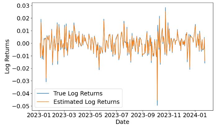
KO stock price 2023-2024: true log returns vs estimated Kalman log returns

This plot shows that KF can predict the KO log returns with very reasonable accuracy.

Minimal 1D Kalman Filter

In this section, we will look at minkf – minimal Kalman filter in Python. This is a minimal implementation with only Numpy dependency.
We generate some 1D random walk data and reconstruct it with KF. The forward and observation models are just identities. The user can either give the model and error covariance matrices as lists, which enable using different values for each time step. If the matrices are given as constant Numpy arrays, the same matrices are used for every time step:

import numpy as np
import minkf as kf
import matplotlib.pyplot as plt

y = np.cumsum(np.random.standard_normal(100))

x0 = np.array([0.0])
Cest0 = 1*np.array([[1.0]])

M = np.array([[1.0]])
K = np.array([[1.0]])
Q = 0.1*np.array([[1.0]])
R = 0.8*np.array([[1.0]])

from IPython.core.display import display, HTML
display(HTML("<style>div.output_scroll { height: 90em; }</style>"))

res = kf.run_filter(y, x0, Cest0, M, K, Q, R, likelihood=True)
res_smo = kf.run_smoother(y, x0, Cest0, M, K, Q, R)

plt.figure(figsize=(10,6))
plt.title('1D Random Walk Data vs Kalman Filter Q=0.1, R=0.8')
plt.rcParams.update({'font.size': 14})
plt.xlabel('Time Step')
plt.plot(y, 'bo', ms=5)
plt.plot(res['x'], 'k-')
plt.plot(res_smo['x'], 'r-')
plt.legend(["Measurements", "True State","Kalman Filter"], loc="lower right")
plt.grid(True)
plt.show()

1D random walk data vs Kalman filter with Q=0.1 and R=0.8

Result is a dict that contains the estimated states and the filtering/smoothing covariances

res['loglike']
242.04184667513363

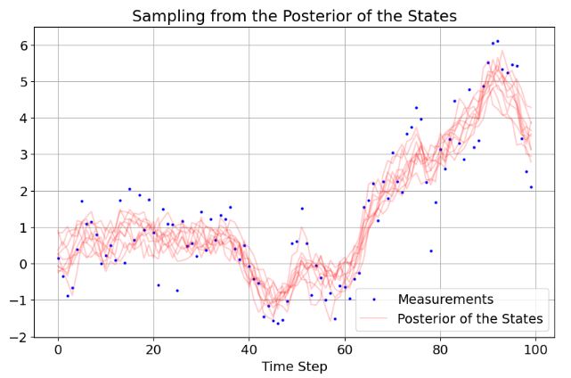
Sampling from the posterior of the states given all the data can be done via the sample function. Sampling needs the KF results, the dynamics model matrix and model error covariance:

samps = kf.sample(res, M, Q, nsamples=10)

from IPython.core.display import display, HTML
display(HTML("<style>div.output_scroll { height: 90em; }</style>"))


plt.figure(figsize=(10,6))
plt.rcParams.update({'font.size': 14})
plt.title('Sampling from the Posterior of the States')
plt.xlabel('Time Step')
plt.plot(y, 'bo', ms=2)
plt.plot(np.array(samps).T, 'r-', alpha=0.2)

plt.legend(["Measurements", "Posterior of the States"], loc="lower right")
plt.grid(True)
plt.show()

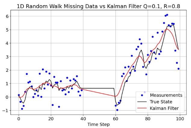
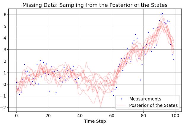
Sampling from the Posterior of the States.

If any element of the observation vector is np.nan, the observation is considered missing. Below is the above simple example with some missing observations in the middle:

y_missing = y.copy()
y_missing[40:60] = np.nan

res_missing = kf.run_filter(y_missing, x0, Cest0, M, K, Q, R, likelihood=True)
res_smo_missing = kf.run_smoother(y_missing, x0, Cest0, M, K, Q, R)

from IPython.core.display import display, HTML
display(HTML("<style>div.output_scroll { height: 90em; }</style>"))



plt.figure(figsize=(10,6))

plt.title('1D Random Walk Missing Data vs Kalman Filter Q=0.1, R=0.8')
plt.rcParams.update({'font.size': 14})
plt.xlabel('Time Step')

plt.plot(y_missing, 'bo', ms=5)
plt.plot(res_missing['x'], 'k-')
plt.plot(res_smo_missing['x'], 'r-')
plt.legend(["Measurements", "True State","Kalman Filter"], loc="lower right")
plt.grid(True)
plt.show()

1D Random Walk Missing Data vs Kalman Filter Q=0.1, R=0.8

from IPython.core.display import display, HTML
display(HTML("<style>div.output_scroll { height: 90em; }</style>"))


samps_missing = kf.sample(res_missing, M, Q, nsamples=10)

plt.figure(figsize=(10,6))
plt.plot(y_missing, 'bo', ms=2)
plt.plot(np.array(samps_missing).T, 'r-', alpha=0.2)
plt.rcParams.update({'font.size': 14})
plt.xlabel('Time Step')
plt.title('Missing Data: Sampling from the Posterior of the States')

plt.legend(["Measurements", "Posterior of the States"], loc="lower right")
plt.grid(True)
plt.show()

1D Kalman Smoothing

This section will deal with tsmoothie – a Python library for time-series smoothing and outlier detection in a vectorized way. This library computes, in a fast and efficient way, the smoothing of single or multiple time-series. The smoothing technique available is Kalman Smoothing with customizable components (level, trend, seasonality, and long seasonality).
In this example, we generate 3 random walk time series of length 100 and apply the Kalman Smoother

import numpy as np
import matplotlib.pyplot as plt
from tsmoothie.smoother import *
from tsmoothie.utils_func import sim_randomwalk

# generate 3 randomwalks timeseries of lenght 100
np.random.seed(123)
data = sim_randomwalk(n_series=3, timesteps=100, 
                      process_noise=10, measure_noise=30)

# operate smoothing
smoother = KalmanSmoother(component='level_trend', 
                          component_noise={'level':0.1, 'trend':0.1})
smoother.smooth(data)

# generate intervals
low, up = smoother.get_intervals('kalman_interval', confidence=0.05)

# plot the first smoothed timeseries with intervals
plt.figure(figsize=(11,6))
plt.plot(smoother.data[0], '.k')
plt.plot(smoother.smooth_data[0], linewidth=3, color='blue')

plt.fill_between(range(len(smoother.data[0])), low[0], up[0], alpha=0.3)
plt.rcParams.update({'font.size': 14})
plt.xlabel('Time Step')
plt.title('Random Walk Data: Kalman Smoothing')

plt.legend(["Measurements", "Kalman Smoother"], loc="lower right")

1D Kalman Time-Series Prediction

Let’s test the function kalman_filter that estimates hidden states using KF:

import numpy as np
import matplotlib.pyplot as plt

# Function to perform Kalman filtering
def kalman_filter(Y, U, Phi, Ypsilon, A, R, Q, x0, P0):
    num_obs = len(Y)
    num_hidden = len(x0)

    # Initialize arrays to store results
    x_pred = np.zeros((num_obs, num_hidden))
    P_pred = np.zeros((num_obs, num_hidden, num_hidden))
    x_filt = np.zeros((num_obs, num_hidden))
    P_filt = np.zeros((num_obs, num_hidden, num_hidden))

    x_pred[0] = x0
    P_pred[0] = P0

    for t in range(1, num_obs):
        # Prediction step
        x_pred[t] = Ypsilon.T * U[t] + Phi[t] @ x_filt[t - 1]
        P_pred[t] = Phi[t] * P_filt[t - 1] * Phi[t].T + Q

        # Kalman gain
        K = P_pred[t] @ A.T @ np.linalg.inv(A @ P_pred[t] @ A.T + R)

        # Update step
        x_filt[t] = x_pred[t] + K @ (Y[t] - A @ x_pred[t])
        P_filt[t] = P_pred[t] - K @ A @ P_pred[t]

    return x_filt, P_filt, x_pred, P_pred

Consider the example of random 1D data

# Example data
num_obs = 1000
num_hidden = 3
np.random.seed(1)

# Simulate exogenous variable U_t
U = np.random.randn(num_obs).T

Applying KF to the simulated data and plotting the result

# Specify matrices in model
A = np.array([[1, 1, 0], [0, 0, 1]])
Phi = np.array([np.array([[0, 0, 0], [0, 0.1, 0], [0, -0.1, 0]]) * np.random.standard_normal() for _ in range(num_obs)]) + np.eye(3)
Q = np.array([[1, 0], [0, 1], [-1, -1]])@np.transpose(np.array([[1, 0], [0, 1], [-1, -1]]))
R = np.eye(2) # Assuming the noise in the observed states is uncorrelated
Ypsilon = np.array([[0.2, 0.25, 0.15]]).T

# Simulate variables v, w, X and Y
v = np.random.multivariate_normal(np.zeros(2), R, num_obs)
w = np.random.multivariate_normal(np.zeros(num_hidden), Q, num_obs)
X = np.zeros((num_obs, num_hidden))
for t in range(1, num_obs):
    X[t] = (Ypsilon.T * U[t] + Phi[t] @ X[t - 1] + w[t])[0]
Y = np.tensordot(A, X, axes=(1,1)).T + v

# Initial state estimate and covariance
x0 = np.zeros(num_hidden)
P0 = Q.copy()


# Estimate hidden states using Kalman filter
x_filt, p_filt, x_pred, p_pred = kalman_filter(Y, U, Phi, Ypsilon, A, R, Q, x0, P0)
plt.figure(figsize=(10,6))
plt.plot(x_filt[:, 0])
plt.fill_between(range(num_obs), x_filt[:, 0] - 1.96*p_filt[:, 0, 0]**.5, x_filt[:, 0] + 1.96*p_filt[:, 0, 0]**.5, alpha=.4)
plt.plot(X[:, 0])
plt.rcParams.update({'font.size': 14})
plt.xlabel('Time Step')
plt.title('Kalman Prediction of Random  Exogenous Data')
plt.legend(['X_predict', 'X_real', 'Confidence bound'])
plt.show()

Kalman Prediction of Random Exogenous Data

This simulation test confirms the validity and effectiveness of using a KF state-space model in 1D time series predictions.

Summary

Kalman filter (KF) is a powerful algorithm that can be employed in the state estimation problems with low signal-to-noise ratio.
This post provided a gentle introduction to the 1D KF, a numerical method that is very popular in time series econometrics.
The aim of the project was to understand the basics of KF in the form of hands-on numerical examples so we could move on to real-world 2D object tracking to be discussed elsewhere.
In the case of a 1D linear system with measurements errors drawn from a random noise KF has been shown to be the robust estimator.
The same approach can be implemented to estimate and cancel out the noise of time-variant signals such as stocks, voltage, ECG, GPS, etc. Also, it can be applied to sensor fusion.
As we saw in our numerical simulations, KF can be incorporated whenever we need to predict the next state of a system based on some noisy measurements.
In the case if nonlinear systems, the extended KF (EKF) which is a nonlinear version of KF should be considered.

References

Go back

Your message has been sent

Make a one-time donation

Make a monthly donation

Make a yearly donation

Choose an amount

€5.00

€15.00

€100.00

€5.00

€15.00

€100.00

€5.00

€15.00

€100.00

Or enter a custom amount

€

Your contribution is appreciated.

Donate Donate monthly Donate yearly

Anatomy of the Robust 1D Kalman Filter

A Simple 1D Voltage Reading

Linear True State & Random Noise

1D Object Tracking

1D State Space Models and Kalman Filtering

KO Log Returns

Minimal 1D Kalman Filter

1D Kalman Smoothing

1D Kalman Time-Series Prediction

Summary

References

Your message has been sent

Make a one-time donation

Make a monthly donation

Make a yearly donation

Discover more from Our Blogs

Leave a comment Cancel reply

Anatomy of the Robust 1D Kalman Filter

A Simple 1D Voltage Reading

Linear True State & Random Noise

1D Object Tracking

1D State Space Models and Kalman Filtering

KO Log Returns

Minimal 1D Kalman Filter

1D Kalman Smoothing

1D Kalman Time-Series Prediction

Summary

References

Your message has been sent

Make a one-time donation

Make a monthly donation

Make a yearly donation

Share this:

Discover more from Our Blogs

Leave a comment Cancel reply

Discover more from Our Blogs