
- In this post, we will take a deep dive into issues around predictive uncertainties of Time Series Forecasting (TSF) models. Our final goal is to minimize decision-making risks.
- TSF is a prediction of what will occur in the future, and it is an uncertain process. Because of the uncertainty, the accuracy of a forecast is as important as the outcome predicted by the TSF model.
- In this study, we’ll examine various sources of TSF, explain common Time Series Analysis (TSA) techniques, and compare different statistical vs Machine Learning (ML) approaches to forecasting.
- The sources of time series data and thus business applications of interest are many: stock prices/returns, airline passengers, housing data, federal funds rate, CO2 concentration, meteorology, sales, oil production, livestock, hotel visitors, market sentiment, etc. The different sources produce observations at different levels of detail and accuracy.
- We will only consider time series that are observed at regular intervals of time (e.g., hourly, daily, weekly, monthly, quarterly, annually). Irregularly spaced time series can also occur, but are beyond the scope of this article.
Table of Contents
- Introduction
- Random Simulation Tests
- TSLA Stock 43 Days
- TSLA Stock 300 Days
- Housing in the United States
- Industrial Production
- Federal Funds Rate Data
- S&P 500 Absolute Returns
- Number of Airline Passengers- 1. Holt-Winters
- Number of Airline Passengers- 2. Prophet
- Average Temperature in India
- Monthly Sales Data Analysis
- QC Audit of Rossmann Stores
- Rossmann Sales Forecasting – 1. Prophet
- Rossmann Sales Forecasting – 2. SARIMA
- CO2 Concentration Data – 1. SARIMA Predictions
- CO2 Concentration Data – 2. ARIMA Dynamic Forecast
- CO2 Concentration Data – 3. ML Regression
- Unemployment/Interest Rate OLS
- Oil Production in Saudi Arabia
- Air Pollution & the Holt’s Method
- Livestock, Sheep in Asia
- International Visitor Nights in Australia
- Hourly Energy Demand Forecasting
- Stock Price Forecasting – 1. TSLA
- Stock Price Forecasting – 2. KO
- FinTech Sentiment Analysis
- Discussion
- Conclusions
- Hands-On TSA(F) Tutorials
- Explore More
Introduction
- TSF is a data science technique that utilizes historical and current data to predict future values over a period of time or a specific point in the future. By analyzing data that we stored in the past, we can make informed decisions that can guide our business strategy and help us understand future trends.
- The most crucial step when considering TSF is understanding your data model and knowing which business questions need to be answered using this data.
- Here, TSA techniques come in handy. TSA isn’t about predicting the future; instead, it’s about understanding the past. It allows developers to decompose data into its constituent parts – trend, seasonality, and residual components. This can help identify any anomalies or shifts in the pattern over time.
- There are three types of TSF: univariate, bivariate, and multivariate forecasting.
- TSF can broadly be categorized into the following categories: statistical models, ML, and Deep Learning (DL).
- We will follow the following 4 steps of TSF: (1) Choosing the desired level of accuracy; (2) defining the business goal(s); (3) time series data mining and TSA; (4) how often model output needed.
- Some common business applications of TSF are predicting the weather, forecasting stock price changes, demand prediction, macro-economic planning, etc.
Random Simulation Tests
- We begin mastering TSF with Autoregressive (AR) Models.
- Let’s set the working directory YOURPATH, import key libraries, simulate stock data as a random sequence, and plot the data
import os
os.chdir('YOURPATH')    # Set working directory
os. getcwd()
import numpy as np
import pandas as pd
import matplotlib.pyplot as plt

# Generate a random time series data
np.random.seed(123)
n_samples = 100
time = pd.date_range('2023-01-01', periods=n_samples, freq='D')
data = np.random.normal(0, 1, n_samples).cumsum()

# Create a DataFrame with the time series data
df = pd.DataFrame({'Time': time, 'Data': data})
df.set_index('Time', inplace=True)

# Plot the time series data
plt.figure(figsize=(10, 4))
plt.plot(df.index, df['Data'])
plt.xlabel('Time')
plt.ylabel('Data')
plt.title('Example Time Series Data')
plt.show()

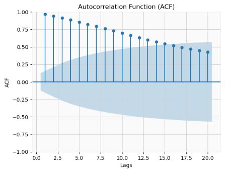
- Plotting ACF
from statsmodels.graphics.tsaplots import plot_acf

# ACF plot
plot_acf(df['Data'], lags=20, zero=False)
plt.xlabel('Lags')
plt.ylabel('ACF')
plt.title('Autocorrelation Function (ACF)')
- Plotting PACF
from statsmodels.graphics.tsaplots import plot_pacf

plot_pacf(df['Data'], lags=20, zero=False)
plt.xlabel('Lags')
plt.ylabel('PACF')
plt.title('Partial Autocorrelation Function (PACF)')
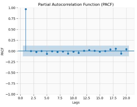
- We can see that ACF is gradually declining with lags. The PACF has 1 significant lag and gradually falling ACF. This means that the data is and AR(1) process.
- Fitting AutoReg models with different orders and comparing AIC and BIC
from statsmodels.tsa.ar_model import AutoReg
max_order = 10
aic_values = []
bic_values = []

for p in range(1, max_order + 1):
    model = AutoReg(data, lags=p)
    result = model.fit()
    aic_values.append(result.aic)
    bic_values.append(result.bic)

# Plot AIC and BIC values
order = range(1, max_order + 1)
plt.plot(order, aic_values, marker='o', label='AIC')
plt.plot(order, bic_values, marker='o', label='BIC')
plt.xlabel('Order (p)')
plt.ylabel('Information Criterion Value')
plt.title('Comparison of AIC and BIC')
plt.legend()
plt.show()
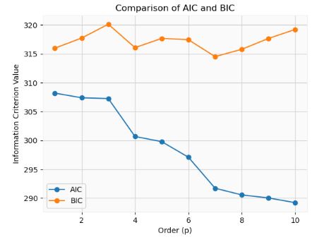
- The model with the lowest AIC or BIC value is often considered the best-fitting model.
- By examining the Ljung-Box test results for different lags, we can determine the appropriate order (p)
import numpy as np
from statsmodels.tsa.ar_model import AutoReg
from statsmodels.stats.diagnostic import acorr_ljungbox

max_order = 10
p_values = []

for p in range(1, max_order + 1):
    model = AutoReg(data, lags=p)
    result = model.fit()
    residuals = result.resid

    result = acorr_ljungbox(residuals, lags=[p])
    p_value = result.iloc[0,1]
    p_values.append(p_value)

# Find the lag order with non-significant autocorrelation
threshold = 0.05
selected_order = np.argmax(np.array(p_values) < threshold) + 1
print("P Values: ", p_values)
print("Selected Order (p):", selected_order)

P Values:  [0.6768877467795985, 0.9665450680852156, 0.2666153891802318, 0.9449353921040547, 0.9017991400094321, 0.9970732878539437, 0.9995994991323243, 0.9978831036372233, 0.986794476112608, 0.9813761718751872]
Selected Order (p): 1
- Cross-validation is another technique for determining the appropriate order (p)
import numpy as np
from statsmodels.tsa.ar_model import AutoReg
from sklearn.metrics import mean_squared_error
from sklearn.model_selection import TimeSeriesSplit

np.random.seed(123)
data = np.random.normal(size=100)

max_order = 9
best_order = None
best_mse = np.inf

tscv = TimeSeriesSplit(n_splits=5)
for p in range(1, max_order + 1):
    mse_scores = []

    for train_index, test_index in tscv.split(data):
        train_data, test_data = data[train_index], data[test_index]

        model = AutoReg(train_data, lags=p)
        result = model.fit()
        predictions = result.predict(start=len(train_data), end=len(train_data) + len(test_data) - 1)

        mse = mean_squared_error(test_data, predictions)
        mse_scores.append(mse)

    avg_mse = np.mean(mse_scores)

    if avg_mse < best_mse:
        best_mse = avg_mse
        best_order = p

print("Best Lag Order (p):", best_order)
Best Lag Order (p): 3
- Here, we choose the lag order (p) that yields the best average performance across the folds.
- Let’s look at a joint distribution of the time series data. If a time series is stationary, then its joint distribution with its lags should be time-invariant. In other words, the distribution should not change as the time index changes.
import seaborn as sns
lag = 10

# stack them into 2D arr
random_process=data1['Close']
joint = np.vstack([random_process[:-lag], random_process[lag:]])
joint0=joint[0]
joint1=joint[1]

df0 = pd.DataFrame({'joint0': joint[0], 'joint1': joint[1]})

sns.jointplot(data=df0, x='joint0', y='joint1', kind="kde")
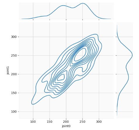
- The joint distribution calculates the likelihood of two events occurring at the same time. A time series represents one possible outcome of a random process that can be completely characterized by its full joint probability distribution, which encompasses all possible combinations of values that the random process can take over an infinite period of time.
TSLA Stock 43 Days
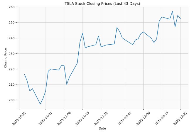
- Let’s apply the above AR approach to the actual TSLA Stock Closing Prices (Last 43 Days)
import datetime
import numpy as np
import yfinance as yf
import matplotlib.pyplot as plt
from sklearn.metrics import mean_squared_error
from sklearn.model_selection import TimeSeriesSplit
from statsmodels.tsa.ar_model import AutoReg
from statsmodels.graphics.tsaplots import plot_acf, plot_pacf
from statsmodels.stats.diagnostic import acorr_ljungbox

ticker = "TSLA"
end_date = datetime.datetime.now().date()
start_date = end_date - datetime.timedelta(days=60)
data3 = yf.download(ticker, start=start_date, end=end_date)
closing_prices = data3["Close"]
print(len(closing_prices))

[*********************100%%**********************]  1 of 1 completed
43

plt.figure(figsize=(10, 6))
plt.plot(closing_prices)
plt.title("TSLA Stock Closing Prices (Last 43 Days)")
plt.xlabel("Date")
plt.ylabel("Closing Price")
plt.xticks(rotation=45)
plt.grid(True)
plt.show()
- Let’s create the 1-day AR(p) forecast as a function of p
n_test = 1
train_data = closing_prices[:len(closing_prices)-n_test]
test_data = closing_prices[len(closing_prices)-n_test:]
print(test_data)

Date
2023-12-22    252.539993
Name: Close, dtype: float64

error_list = []
for i in range(1,11):
    model = AutoReg(train_data, lags=i)
    model_fit = model.fit()
    predicted_price = float(model_fit.predict(start=len(train_data), end=len(train_data)))
    actual_price = test_data.iloc[0]
    error_list.append(abs(actual_price - predicted_price))

plt.figure(figsize=(10, 6))
plt.plot(error_list)
plt.title("Errors (Actual - Predicted)")
plt.xlabel("p")
plt.ylabel("Error")
plt.xticks(rotation=45)
plt.grid(True)
plt.show()
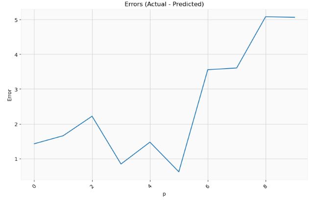
- It is clear that the optimal p-value is p=5.
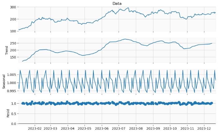
- Implementing the statsmodels seasonal decomposition of our time series data. This decomposition separates a time series into three distinct components: trend, seasonality, and residual (or irregular) component. Understanding these components helps in understanding underlying patterns in the data, forecasting, and making business or economic decisions.
import numpy as np
import pandas as pd
from statsmodels.tsa.seasonal import seasonal_decompose
y = pd.Series(df["Data"], df.index)
result = seasonal_decompose(y, model='multiplicative',period=10)

fig=result.plot()
fig.set_size_inches((10, 6))
- Performing the ADF test of stationarity
from statsmodels.tsa.stattools import adfuller

ts_stationary=pd.Series(data=y, index=df.index)

result = adfuller(ts_stationary)
print(result)

print('ADF Statistic: %f' % result[0])
print('p-value: %f' % result[1])

(-2.4007209950719894, 0.14153301655714257, 4, 241, {'1%': -3.4577787098622674, '5%': -2.873608704758507, '10%': -2.573201765981991}, 1549.8412743269414)
ADF Statistic: -2.400721
p-value: 0.141533
- Since the p-value is higher than 0.05 significance level, we can accept the null hypothesis, and the time series is not stationary.
- Let’s check the stability of the model over time by computing the rolling mean and variance
rolling_mean_s = ts_stationary.rolling(window=5).mean()
rolling_var_s = ts_stationary.rolling(window=5).var()

plt.plot(rolling_mean_s, label="Rolling Mean")
plt.plot(rolling_var_s, label="Rolling Variance")
plt.legend(loc="best")
plt.title("Rollings Stationary")
plt.show()

- Performing the KPSS test of stationarity. This test figures out if a time series is stationary around a mean or linear trend, or is non-stationary due to a unit root. A stationary time series is one where statistical properties – like the mean and variance – are constant over time.
from statsmodels.tsa.stattools import kpss
result = kpss(ts_stationary, regression='c')
print('KPSS Statistic: %f' % result[0])
print('p-value: %f' % result[1])
KPSS Statistic: 1.385231
p-value: 0.010000
- Here, a p-value of 0.01 (1%) would cause the null hypothesis to be rejected at an alpha level of 0.05 (5%).
- Seasonal-Trend decomposition using LOESS (STL)
from statsmodels.tsa.seasonal import STL
result = STL(mydata, period=12, seasonal=7, robust=True).fit()
plt.figure(figsize=(11, 7))
plt.subplot(411)
plt.plot(mydata, label='Original')
plt.legend(loc='best')
plt.subplot(412)
plt.plot(result.trend, label='Trend')
plt.legend(loc='best')
plt.subplot(413)
plt.plot(result.seasonal,label='Seasonality')
plt.legend(loc='best')
plt.subplot(414)
plt.plot(result.resid, label='Residuals')
plt.legend(loc='best')
plt.tight_layout()
plt.show()
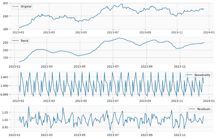
- Loess is not a decomposition method, but rather a smoothing method. The STL algorithm uses the Loess algorithm as a step in computing the seasonal decomposition.
TSLA Stock 300 Days
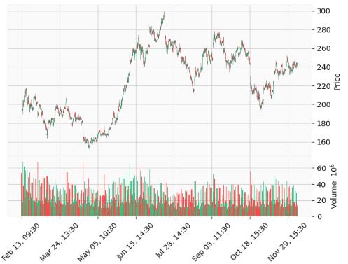
- Let’s use yfinance to download the TSLA stock data with days=300 and interval=’1h’
import ta
import talib
import yfinance as yf
import mplfinance as mpf
import matplotlib.pyplot as plt
from datetime import datetime, timedelta

ticker = "TSLA"

end_date = datetime.today().strftime('%Y-%m-%d')
start_date = (datetime.today() - timedelta(days=300)).strftime('%Y-%m-%d')

data = yf.download(ticker, start=start_date, end=end_date, interval='1h')
[*********************100%***********************]  1 of 1 completed

mpf.plot(data, type='candle', volume=True, style='yahoo')
- Importing key libraries and plotting PACF/ACF of Close Price
from statsmodels.graphics.tsaplots import plot_pacf
from statsmodels.graphics.tsaplots import plot_acf
from statsmodels.tsa.statespace.sarimax import SARIMAX
from statsmodels.tsa.holtwinters import ExponentialSmoothing
from statsmodels.tsa.stattools import adfuller
import matplotlib.pyplot as plt
from tqdm import tqdm_notebook
import numpy as np
import pandas as pd

from itertools import product

import warnings
warnings.filterwarnings('ignore')

%matplotlib inline
plot_pacf(data['Close']);
plot_acf(data['Close']);
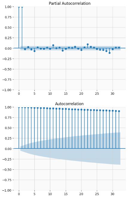
- The ADF test confirms that the dataset is not stationary
# Augmented Dickey-Fuller test

ad_fuller_result = adfuller(data['Close'])
print(f'ADF Statistic: {ad_fuller_result[0]}')
print(f'p-value: {ad_fuller_result[1]}')

ADF Statistic: -1.5485859095622545
p-value: 0.5093544755020373
- Taking the log-domain 1st difference transformation to make the data stationary
data['data'] = np.log(data['Close'])
data['data'] = data['Close'].diff()
data = data.drop(data.index[0])

plt.figure(figsize=[15, 7.5]);
plt.plot(data['data'])
plt.title("Log Difference of Close Price for TSLA")
plt.show()
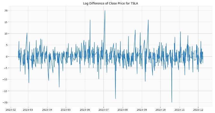
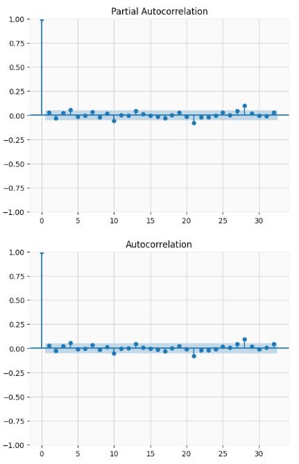
- Both the ADF test and PACF/ACF confirm that the transformed dataset is stationary
ad_fuller_result = adfuller(data['data'])
print(f'ADF Statistic: {ad_fuller_result[0]}')
print(f'p-value: {ad_fuller_result[1]}')

ADF Statistic: -17.738476868990166
p-value: 3.410415880267577e-30

plot_pacf(data['data']);
plot_acf(data['data']);
- Optimizing the SARIMAX model parameters
def optimize_SARIMA(parameters_list, d, D, s, exog):
    """
        Return dataframe with parameters, corresponding AIC and SSE

        parameters_list - list with (p, q, P, Q) tuples
        d - integration order
        D - seasonal integration order
        s - length of season
        exog - the exogenous variable
    """

    results = []

    for param in tqdm_notebook(parameters_list):
        try:
            model = SARIMAX(exog, order=(param[0], d, param[1]), seasonal_order=(param[2], D, param[3], s)).fit(disp=-1)
        except:
            continue

        aic = model.aic
        results.append([param, aic])

    result_df = pd.DataFrame(results)
    result_df.columns = ['(p,q)x(P,Q)', 'AIC']
    #Sort in ascending order, lower AIC is better
    result_df = result_df.sort_values(by='AIC', ascending=True).reset_index(drop=True)

    return result_df

p = range(0, 4, 1)
d = 1
q = range(0, 4, 1)
P = range(0, 4, 1)
D = 1
Q = range(0, 4, 1)
s = 4

parameters = product(p, q, P, Q)
parameters_list = list(parameters)
print(len(parameters_list))
256
result_df = optimize_SARIMA(parameters_list, 1, 1, 4, data['data'])
result_df

0%|          | 0/256 [00:00<?, ?it/s]
(p,q)x(P,Q)	AIC
0	(3, 3, 0, 0)	14.000000
1	(1, 2, 0, 2)	6838.178237
2	(1, 2, 1, 1)	6838.344379
3	(0, 1, 2, 3)	6839.006923
4	(0, 1, 3, 3)	6839.726108
...	...	...
251	(2, 0, 0, 0)	8147.031496
252	(0, 0, 2, 0)	8201.217015
253	(1, 0, 0, 0)	8307.942745
254	(0, 0, 1, 0)	8362.245368
255	(0, 0, 0, 0)	8688.024189
256 rows × 2 columns

best_model = SARIMAX(data['data'], order=(3, 3, 0)).fit(dis=-1)
print(best_model.summary())

SARIMAX Results
==============================================================================
Dep. Variable:                   data   No. Observations:                 1450
Model:               SARIMAX(3, 3, 0)   Log Likelihood               -4440.140
Date:                Sun, 10 Dec 2023   AIC                           8888.280
Time:                        13:36:39   BIC                           8909.389
Sample:                             0   HQIC                          8896.158
                               - 1450
Covariance Type:                  opg
==============================================================================
                 coef    std err          z      P>|z|      [0.025      0.975]
------------------------------------------------------------------------------
ar.L1         -1.4624      0.020    -74.995      0.000      -1.501      -1.424
ar.L2         -1.1894      0.029    -41.353      0.000      -1.246      -1.133
ar.L3         -0.5277      0.023    -23.438      0.000      -0.572      -0.484
sigma2        27.0414      0.746     36.225      0.000      25.578      28.505
===================================================================================
Ljung-Box (L1) (Q):                  82.80   Jarque-Bera (JB):               780.60
Prob(Q):                              0.00   Prob(JB):                         0.00
Heteroskedasticity (H):               1.45   Skew:                            -0.07
Prob(H) (two-sided):                  0.00   Kurtosis:                         6.60
===================================================================================
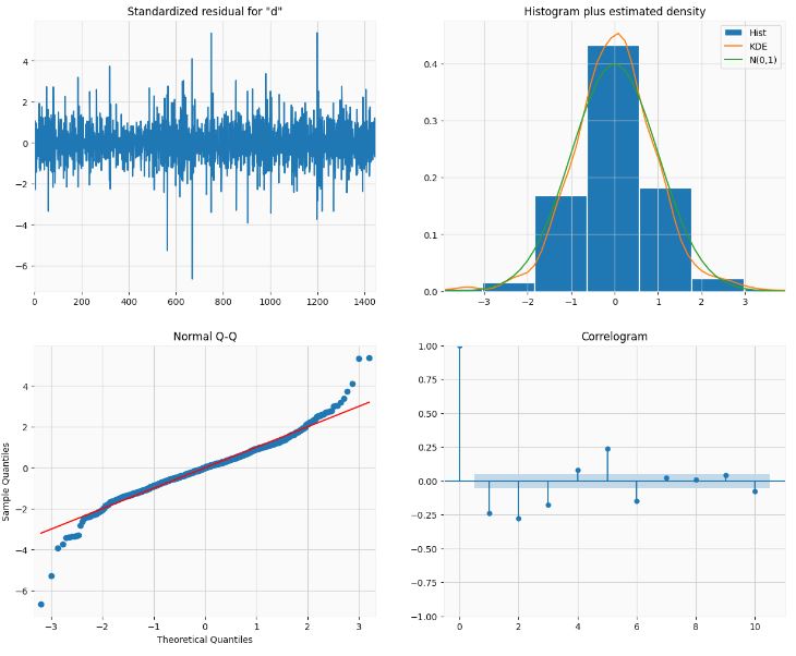
- Plotting the best SARIMAX model diagnostics
best_model.plot_diagnostics(figsize=(15,12));
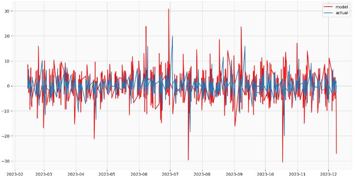
- Creating and plotting the best SARIMAX model forecast
data['arima_model'] = best_model.fittedvalues
data['arima_model'][:4+1] = np.NaN

forecast = best_model.predict(start=data.shape[0], end=data.shape[0] + 8)
forecast = data['arima_model'].append(forecast)
forecast1=forecast[9:]
df = pd.DataFrame({'Time': data.index, 'Data': forecast1})
df.set_index('Time', inplace=True)
plt.figure(figsize=(15, 7.5))
plt.plot(data.index,forecast1, color='r', label='model')
plt.plot(data.index,data['data'], label='actual')
plt.legend()

plt.show()
Housing in the United States
- Let’s apply the AR approach to the month-over-month growth rate in U.S. Housing
%matplotlib inline
import matplotlib.pyplot as plt
import pandas as pd
import pandas_datareader as pdr
import seaborn as sns
from statsmodels.tsa.api import acf, graphics, pacf
from statsmodels.tsa.ar_model import AutoReg, ar_select_order
sns.set_style("darkgrid")
pd.plotting.register_matplotlib_converters()
# Default figure size
sns.mpl.rc("figure", figsize=(16, 6))
sns.mpl.rc("font", size=14)
data = pdr.get_data_fred("HOUSTNSA", "1959-01-01", "2023-12-24")
housing = data.HOUSTNSA.pct_change().dropna()
# Scale by 100 to get percentages
housing = 100 * housing.asfreq("MS")
fig, ax = plt.subplots()
ax = housing.plot(ax=ax)
- Let’s examine the AutoReg Model Results
mod = AutoReg(housing, 3, old_names=False)
res = mod.fit()
print(res.summary())
  AutoReg Model Results
==============================================================================
Dep. Variable:               HOUSTNSA   No. Observations:                  778
Model:                     AutoReg(3)   Log Likelihood               -3198.885
Method:               Conditional MLE   S.D. of innovations             15.009
Date:                Sat, 23 Dec 2023   AIC                           6407.770
Time:                        13:26:45   BIC                           6431.034
Sample:                    05-01-1959   HQIC                          6416.720
                         - 11-01-2023
===============================================================================
                  coef    std err          z      P>|z|      [0.025      0.975]
-------------------------------------------------------------------------------
const           1.0998      0.543      2.027      0.043       0.036       2.163
HOUSTNSA.L1     0.1835      0.035      5.211      0.000       0.114       0.253
HOUSTNSA.L2     0.0080      0.036      0.223      0.823      -0.062       0.078
HOUSTNSA.L3    -0.1950      0.035     -5.549      0.000      -0.264      -0.126
                                    Roots
=============================================================================
                  Real          Imaginary           Modulus         Frequency
-----------------------------------------------------------------------------
AR.1            0.9659           -1.3337j            1.6467           -0.1502
AR.2            0.9659           +1.3337j            1.6467            0.1502
AR.3           -1.8908           -0.0000j            1.8908           -0.5000
-----------------------------------------------------------------------------
sel = ar_select_order(housing, 13, old_names=False)
sel.ar_lags
res = sel.model.fit()
print(res.summary())
                           AutoReg Model Results
==============================================================================
Dep. Variable:               HOUSTNSA   No. Observations:                  778
Model:                    AutoReg(13)   Log Likelihood               -2886.312
Method:               Conditional MLE   S.D. of innovations             10.528
Date:                Sat, 23 Dec 2023   AIC                           5802.624
Time:                        13:26:51   BIC                           5872.222
Sample:                    03-01-1960   HQIC                          5829.417
                         - 11-01-2023
================================================================================
                   coef    std err          z      P>|z|      [0.025      0.975]
--------------------------------------------------------------------------------
const            1.4561      0.448      3.250      0.001       0.578       2.334
HOUSTNSA.L1     -0.2665      0.035     -7.710      0.000      -0.334      -0.199
HOUSTNSA.L2     -0.0833      0.031     -2.699      0.007      -0.144      -0.023
HOUSTNSA.L3     -0.0880      0.031     -2.861      0.004      -0.148      -0.028
HOUSTNSA.L4     -0.1724      0.031     -5.623      0.000      -0.233      -0.112
HOUSTNSA.L5     -0.0450      0.031     -1.447      0.148      -0.106       0.016
HOUSTNSA.L6     -0.0907      0.031     -2.963      0.003      -0.151      -0.031
HOUSTNSA.L7     -0.0715      0.031     -2.330      0.020      -0.132      -0.011
HOUSTNSA.L8     -0.1584      0.031     -5.174      0.000      -0.218      -0.098
HOUSTNSA.L9     -0.0898      0.031     -2.887      0.004      -0.151      -0.029
HOUSTNSA.L10    -0.1111      0.031     -3.627      0.000      -0.171      -0.051
HOUSTNSA.L11     0.1036      0.031      3.370      0.001       0.043       0.164
HOUSTNSA.L12     0.5028      0.031     16.303      0.000       0.442       0.563
HOUSTNSA.L13     0.2961      0.035      8.571      0.000       0.228       0.364
                                    Roots
==============================================================================
                   Real          Imaginary           Modulus         Frequency
------------------------------------------------------------------------------
AR.1             1.1036           -0.0000j            1.1036           -0.0000
AR.2             0.8751           -0.5032j            1.0095           -0.0831
AR.3             0.8751           +0.5032j            1.0095            0.0831
AR.4             0.5052           -0.8782j            1.0132           -0.1669
AR.5             0.5052           +0.8782j            1.0132            0.1669
AR.6             0.0126           -1.0588j            1.0589           -0.2481
AR.7             0.0126           +1.0588j            1.0589            0.2481
AR.8            -0.5285           -0.9382j            1.0768           -0.3316
AR.9            -0.5285           +0.9382j            1.0768            0.3316
AR.10           -0.9602           -0.5903j            1.1271           -0.4123
AR.11           -0.9602           +0.5903j            1.1271            0.4123
AR.12           -1.3050           -0.2611j            1.3309           -0.4686
AR.13           -1.3050           +0.2611j            1.3309            0.4686
------------------------------------------------------------------------------
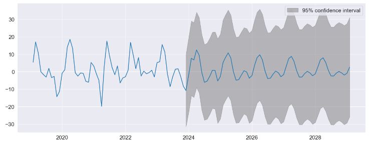
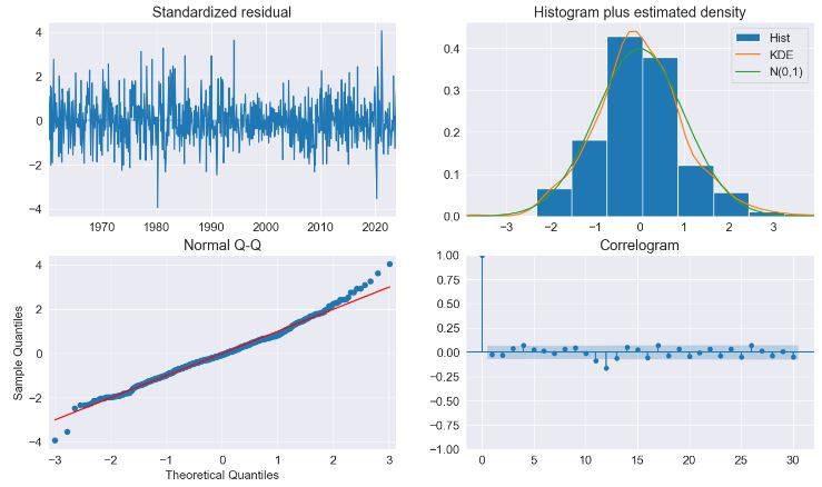
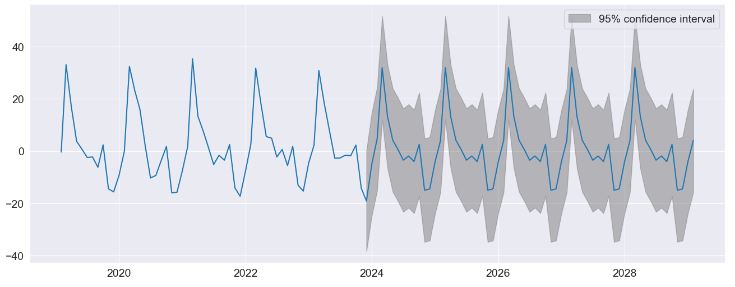
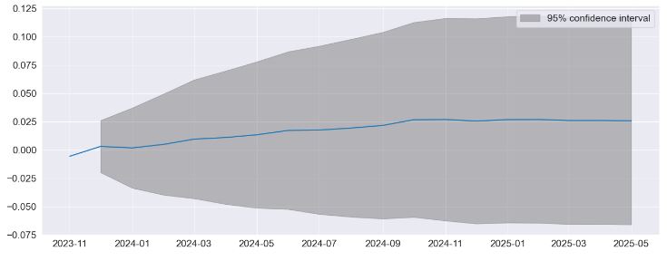
- Performing predictions to show the string seasonality captured by the model with 95% confidence interval
fig = res.plot_predict(720, 840)
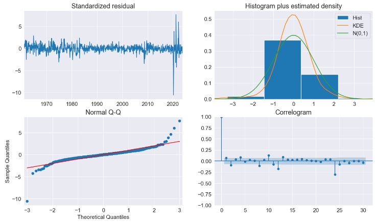
- The key diagnostics plot indicates that the model captures the key features in the data
fig = plt.figure(figsize=(16, 9))
fig = res.plot_diagnostics(fig=fig, lags=30)
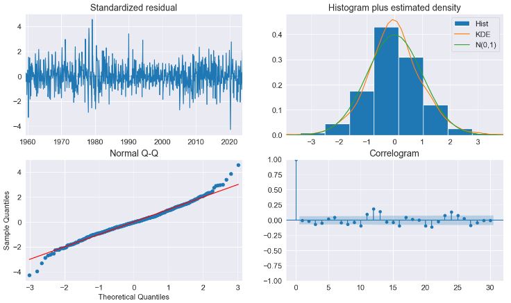
- Testing model predictions with seasonal dummies
sel = ar_select_order(housing, 13, seasonal=True, old_names=False)
sel.ar_lags
res = sel.model.fit()
print(res.summary())
AutoReg Model Results
==============================================================================
Dep. Variable: HOUSTNSA No. Observations: 778
Model: Seas. AutoReg(2) Log Likelihood -2871.089
Method: Conditional MLE S.D. of innovations 9.786
Date: Sat, 23 Dec 2023 AIC 5772.178
Time: 13:27:10 BIC 5841.991
Sample: 04-01-1959 HQIC 5799.036
- 11-01-2023
===============================================================================
coef std err z P>|z| [0.025 0.975]
-------------------------------------------------------------------------------
const 1.5571 1.348 1.155 0.248 -1.085 4.199
s(2,12) 30.9672 1.806 17.149 0.000 27.428 34.506
s(3,12) 19.9295 2.332 8.545 0.000 15.358 24.501
s(4,12) 9.0602 2.561 3.537 0.000 4.040 14.080
s(5,12) 1.3026 2.041 0.638 0.523 -2.697 5.303
s(6,12) -4.5037 1.868 -2.411 0.016 -8.164 -0.843
s(7,12) -4.2775 1.806 -2.369 0.018 -7.816 -0.739
s(8,12) -6.3883 1.773 -3.604 0.000 -9.862 -2.914
s(9,12) -0.1806 1.781 -0.101 0.919 -3.670 3.309
s(10,12) -16.3239 1.790 -9.120 0.000 -19.832 -12.816
s(11,12) -19.4906 1.849 -10.542 0.000 -23.114 -15.867
s(12,12) -10.6999 1.771 -6.042 0.000 -14.171 -7.229
HOUSTNSA.L1 -0.2472 0.036 -6.903 0.000 -0.317 -0.177
HOUSTNSA.L2 -0.0994 0.036 -2.776 0.005 -0.170 -0.029
Roots
=============================================================================
Real Imaginary Modulus Frequency
-----------------------------------------------------------------------------
AR.1 -1.2430 -2.9173j 3.1710 -0.3141
AR.2 -1.2430 +2.9173j 3.1710 0.3141
-----------------------------------------------------------------------------
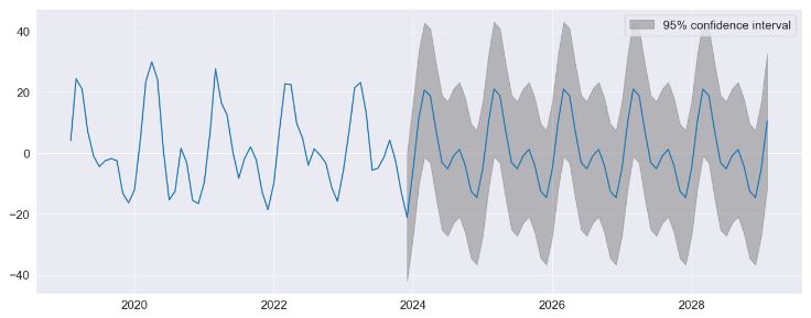
fig = res.plot_predict(720, 840)
fig = plt.figure(figsize=(16, 9))
fig = res.plot_diagnostics(lags=30, fig=fig)
- Implementing the Custom Deterministic Process. This allows for more complex deterministic terms to be constructed, for example one that includes seasonal components with two periods, or one that uses a Fourier series rather than seasonal dummies
from statsmodels.tsa.deterministic import DeterministicProcess

dp = DeterministicProcess(housing.index, constant=True, period=12, fourier=2)
mod = AutoReg(housing, 2, trend="n", seasonal=False, deterministic=dp)
res = mod.fit()
print(res.summary())

                            AutoReg Model Results
==============================================================================
Dep. Variable:               HOUSTNSA   No. Observations:                  778
Model:                     AutoReg(2)   Log Likelihood               -2935.525
Method:               Conditional MLE   S.D. of innovations             10.633
Date:                Sat, 23 Dec 2023   AIC                           5887.049
Time:                        13:29:17   BIC                           5924.283
Sample:                    04-01-1959   HQIC                          5901.373
                         - 11-01-2023
===============================================================================
                  coef    std err          z      P>|z|      [0.025      0.975]
-------------------------------------------------------------------------------
const           1.6591      0.387      4.289      0.000       0.901       2.417
sin(1,12)      15.3251      0.818     18.732      0.000      13.722      16.929
cos(1,12)       4.8543      0.578      8.396      0.000       3.721       5.987
sin(2,12)      11.8657      0.605     19.628      0.000      10.681      13.051
cos(2,12)       0.0660      0.717      0.092      0.927      -1.339       1.471
HOUSTNSA.L1    -0.3403      0.036     -9.571      0.000      -0.410      -0.271
HOUSTNSA.L2    -0.1497      0.036     -4.212      0.000      -0.219      -0.080
                                    Roots
=============================================================================
                  Real          Imaginary           Modulus         Frequency
-----------------------------------------------------------------------------
AR.1           -1.1364           -2.3210j            2.5843           -0.3225
AR.2           -1.1364           +2.3210j            2.5843            0.3225
-----------------------------------------------------------------------------

fig = res.plot_predict(720, 840)
Industrial Production
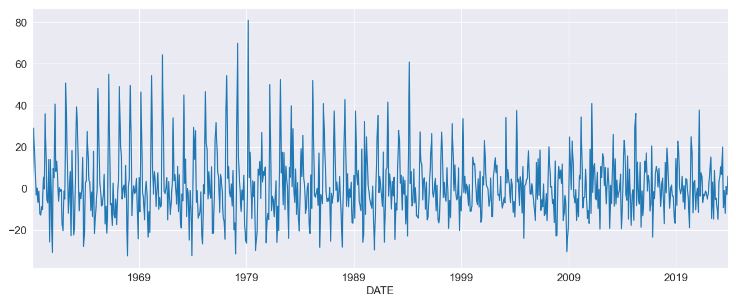
- Let’s apply the AR forecasting to the industrial production index data
data = pdr.get_data_fred("INDPRO", "1959-01-01", "2023-12-24")
ind_prod = data.INDPRO.pct_change(12).dropna().asfreq("MS")
_, ax = plt.subplots(figsize=(16, 9))
ind_prod.plot(ax=ax)

sel = ar_select_order(ind_prod, 13, "bic", old_names=False)
res = sel.model.fit()
print(res.summary())

ind_prod.shape
(767,)
fig = res_glob.plot_predict(start=766, end=784)
res_ar5 = AutoReg(ind_prod, 5, old_names=False).fit()

predictions = pd.DataFrame(
    {
        "AR(5)": res_ar5.predict(start=766, end=784),
        "AR(13)": res.predict(start=766, end=784),
        "Restr. AR(13)": res_glob.predict(start=766, end=784),
    }
)
_, ax = plt.subplots()
ax = predictions.plot(ax=ax)
           AutoReg Model Results
==============================================================================
Dep. Variable:                 INDPRO   No. Observations:                  767
Model:                    AutoReg(13)   Log Likelihood                2293.864
Method:               Conditional MLE   S.D. of innovations              0.012
Date:                Sat, 23 Dec 2023   AIC                          -4557.727
Time:                        13:28:11   BIC                          -4488.347
Sample:                    02-01-1961   HQIC                         -4531.000
                         - 11-01-2023
==============================================================================
                 coef    std err          z      P>|z|      [0.025      0.975]
------------------------------------------------------------------------------
const          0.0015      0.001      2.940      0.003       0.001       0.003
INDPRO.L1      1.2122      0.034     35.403      0.000       1.145       1.279
INDPRO.L2     -0.3039      0.054     -5.589      0.000      -0.411      -0.197
INDPRO.L3      0.1038      0.055      1.889      0.059      -0.004       0.211
INDPRO.L4      0.0310      0.055      0.562      0.574      -0.077       0.139
INDPRO.L5     -0.0866      0.055     -1.578      0.115      -0.194       0.021
INDPRO.L6      0.0501      0.055      0.918      0.359      -0.057       0.157
INDPRO.L7     -0.0037      0.055     -0.067      0.946      -0.111       0.103
INDPRO.L8     -0.0894      0.054     -1.641      0.101      -0.196       0.017
INDPRO.L9      0.1202      0.055      2.205      0.027       0.013       0.227
INDPRO.L10     0.0097      0.055      0.177      0.859      -0.097       0.117
INDPRO.L11    -0.1255      0.054     -2.304      0.021      -0.232      -0.019
INDPRO.L12    -0.3056      0.053     -5.719      0.000      -0.410      -0.201
INDPRO.L13     0.3295      0.033      9.946      0.000       0.265       0.394
                                    Roots
==============================================================================
                   Real          Imaginary           Modulus         Frequency
------------------------------------------------------------------------------
AR.1            -1.0884           -0.3009j            1.1292           -0.4571
AR.2            -1.0884           +0.3009j            1.1292            0.4571
AR.3            -0.8108           -0.8184j            1.1520           -0.3743
AR.4            -0.8108           +0.8184j            1.1520            0.3743
AR.5            -0.2810           -1.0316j            1.0692           -0.2923
AR.6            -0.2810           +1.0316j            1.0692            0.2923
AR.7             0.2883           -1.0171j            1.0572           -0.2060
AR.8             0.2883           +1.0171j            1.0572            0.2060
AR.9             0.7786           -0.7401j            1.0743           -0.1210
AR.10            0.7786           +0.7401j            1.0743            0.1210
AR.11            1.0384           -0.2257j            1.0627           -0.0341
AR.12            1.0384           +0.2257j            1.0627            0.0341
AR.13            1.0771           -0.0000j            1.0771           -0.0000
------------------------------------------------------------------------------

- The diagnostics indicate the model captures most of the the dynamics in the data. The correlogram shows a patters at the seasonal frequency and so a more complete seasonal model (
SARIMAX) may be needed. Read more here. - Let’s produce 12-step-heard forecasts for the final 24 periods in the sample. Forecasts are produced using the
predictmethod from a results instance. The default produces static forecasts which are one-step forecasts. Producing multi-step forecasts requires usingdynamic=True.
import numpy as np

start = ind_prod.index[-24]
forecast_index = pd.date_range(start, freq=ind_prod.index.freq, periods=36)
cols = ["-".join(str(val) for val in (idx.year, idx.month)) for idx in forecast_index]
forecasts = pd.DataFrame(index=forecast_index, columns=cols)
for i in range(1, 24):
    fcast = res_glob.predict(
        start=forecast_index[i], end=forecast_index[i + 12], dynamic=True
    )
    forecasts.loc[fcast.index, cols[i]] = fcast
_, ax = plt.subplots(figsize=(16, 10))
ind_prod.iloc[-24:].plot(ax=ax, color="black", linestyle="--")
ax = forecasts.plot(ax=ax)

- Comparing to SARIMAX
from statsmodels.tsa.api import SARIMAX

sarimax_mod = SARIMAX(ind_prod, order=((1, 5, 12, 13), 0, 0), trend="c")
sarimax_res = sarimax_mod.fit()
print(sarimax_res.summary())

      SARIMAX Results
=========================================================================================
Dep. Variable:                            INDPRO   No. Observations:                  767
Model:             SARIMAX([1, 5, 12, 13], 0, 0)   Log Likelihood                2282.426
Date:                           Sat, 23 Dec 2023   AIC                          -4552.853
Time:                                   13:29:05   BIC                          -4524.998
Sample:                               01-01-1960   HQIC                         -4542.131
                                    - 11-01-2023
Covariance Type:                             opg
==============================================================================
                 coef    std err          z      P>|z|      [0.025      0.975]
------------------------------------------------------------------------------
intercept      0.0015      0.000      3.266      0.001       0.001       0.002
ar.L1          1.0263      0.009    112.105      0.000       1.008       1.044
ar.L5         -0.0306      0.014     -2.198      0.028      -0.058      -0.003
ar.L12        -0.4697      0.010    -49.317      0.000      -0.488      -0.451
ar.L13         0.4159      0.013     32.167      0.000       0.391       0.441
sigma2         0.0002   2.24e-06     67.499      0.000       0.000       0.000
===================================================================================
Ljung-Box (L1) (Q):                  34.68   Jarque-Bera (JB):             18537.97
Prob(Q):                              0.00   Prob(JB):                         0.00
Heteroskedasticity (H):               1.56   Skew:                            -0.98
Prob(H) (two-sided):                  0.00   Kurtosis:                        27.01
===================================================================================

sarimax_params = sarimax_res.params.iloc[:-1].copy()
sarimax_params.index = res_glob.params.index
params = pd.concat([res_glob.params, sarimax_params], axis=1, sort=False)
params.columns = ["AutoReg", "SARIMAX"]
params

	         AutoReg	SARIMAX
const	    0.001517	0.001471
INDPRO.L1	1.172634	1.026293
INDPRO.L2	-0.183711	-0.030650
INDPRO.L12	-0.417311	-0.469672
INDPRO.L13	0.370521	0.415866
Federal Funds Rate Data
- Let’s look at an example of the use of Markov switching models in statsmodels to estimate dynamic regression models with changes in regime. Read the Stata Markov switching documentation here.
- Our first example deals with the Federal funds rate data
from statsmodels.tsa.regime_switching.tests.test_markov_regression import fedfunds
dta_fedfunds = pd.Series(
fedfunds, index=pd.date_range("1954-07-01", "2010-10-01", freq="QS")
)
# Plot the data
dta_fedfunds.plot(title="Federal funds rate", figsize=(12, 3))
# Fit the model
# (a switching mean is the default of the MarkovRegession model)
mod_fedfunds = sm.tsa.MarkovRegression(dta_fedfunds, k_regimes=2)
res_fedfunds = mod_fedfunds.fit()
res_fedfunds.summary()
Markov Switching Model Results
Dep. Variable: y No. Observations: 226
Model: MarkovRegression Log Likelihood -508.636
Date: Sat, 23 Dec 2023 AIC 1027.272
Time: 13:29:47 BIC 1044.375
Sample: 07-01-1954 HQIC 1034.174
- 10-01-2010
Covariance Type: approx
Regime 0 parameters
coef std err z P>|z| [0.025 0.975]
const 3.7088 0.177 20.988 0.000 3.362 4.055
Regime 1 parameters
coef std err z P>|z| [0.025 0.975]
const 9.5568 0.300 31.857 0.000 8.969 10.145
Non-switching parameters
coef std err z P>|z| [0.025 0.975]
sigma2 4.4418 0.425 10.447 0.000 3.608 5.275
Regime transition parameters
coef std err z P>|z| [0.025 0.975]
p[0->0] 0.9821 0.010 94.443 0.000 0.962 1.002
p[1->0] 0.0504 0.027 1.876 0.061 -0.002 0.103
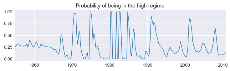
res_fedfunds.smoothed_marginal_probabilities[1].plot(
title="Probability of being in the high regime", figsize=(12, 3)
)
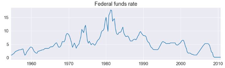
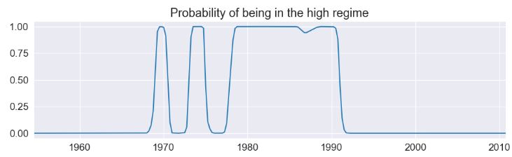
- The model suggests that the 1980’s was a time-period in which a high federal funds rate existed.
- From the estimated transition matrix we can calculate the expected duration of a low regime versus a high regime.
print(res_fedfunds.expected_durations)
[55.85400626 19.85506546]
- The next example augments the previous model to include the lagged value of the federal funds rate
# Fit the model
mod_fedfunds2 = sm.tsa.MarkovRegression(
    dta_fedfunds.iloc[1:], k_regimes=2, exog=dta_fedfunds.iloc[:-1]
)
res_fedfunds2 = mod_fedfunds2.fit()

res_fedfunds2.summary()

Markov Switching Model Results
Dep. Variable:	y	No. Observations:	225
Model:	MarkovRegression	Log Likelihood	-264.711
Date:	Sat, 23 Dec 2023	AIC	543.421
Time:	13:29:57	BIC	567.334
Sample:	10-01-1954	HQIC	553.073
- 10-01-2010
Covariance Type:	approx
Regime 0 parameters
coef	std err	z	P>|z|	[0.025	0.975]
const	0.7245	0.289	2.510	0.012	0.159	1.290
x1	0.7631	0.034	22.629	0.000	0.697	0.829
Regime 1 parameters
coef	std err	z	P>|z|	[0.025	0.975]
const	-0.0989	0.118	-0.835	0.404	-0.331	0.133
x1	1.0612	0.019	57.351	0.000	1.025	1.097
Non-switching parameters
coef	std err	z	P>|z|	[0.025	0.975]
sigma2	0.4783	0.050	9.642	0.000	0.381	0.576
Regime transition parameters
coef	std err	z	P>|z|	[0.025	0.975]
p[0->0]	0.6378	0.120	5.304	0.000	0.402	0.874
p[1->0]	0.1306	0.050	2.634	0.008	0.033	0.228

res_fedfunds2.smoothed_marginal_probabilities[0].plot(
    title="Probability of being in the high regime", figsize=(12, 3)
)
- There are several things to notice from the summary output:
- The information criteria have decreased substantially, indicating that this model has a better fit than the previous model.
- The interpretation of the regimes, in terms of the intercept, have switched. Now the first regime has the higher intercept and the second regime has a lower intercept.
- Examining the smoothed probabilities of the high regime state, we now see quite a bit more variability.
- Finally, the expected durations of each regime have decreased quite a bit.
print(res_fedfunds2.expected_durations)
[2.76105188 7.65529154]
- Taylor rule with 2 or 3 regimes: Let’s include two additional exogenous variables – a measure of the output gap and a measure of inflation – to estimate a switching Taylor-type rule with both 2 and 3 regimes to see which fits the data better.
- Because the models can be often difficult to estimate, for the 3-regime model we employ a search over starting parameters to improve results, specifying 20 random search repetitions.
# Get the additional data
from statsmodels.tsa.regime_switching.tests.test_markov_regression import ogap, inf

dta_ogap = pd.Series(ogap, index=pd.date_range("1954-07-01", "2010-10-01", freq="QS"))
dta_inf = pd.Series(inf, index=pd.date_range("1954-07-01", "2010-10-01", freq="QS"))

exog = pd.concat((dta_fedfunds.shift(), dta_ogap, dta_inf), axis=1).iloc[4:]

# Fit the 2-regime model
mod_fedfunds3 = sm.tsa.MarkovRegression(dta_fedfunds.iloc[4:], k_regimes=2, exog=exog)
res_fedfunds3 = mod_fedfunds3.fit()

# Fit the 3-regime model
np.random.seed(12345)
mod_fedfunds4 = sm.tsa.MarkovRegression(dta_fedfunds.iloc[4:], k_regimes=3, exog=exog)
res_fedfunds4 = mod_fedfunds4.fit(search_reps=20)
res_fedfunds3.summary()
Markov Switching Model Results
Dep. Variable:	y	No. Observations:	222
Model:	MarkovRegression	Log Likelihood	-229.256
Date:	Sat, 23 Dec 2023	AIC	480.512
Time:	13:30:09	BIC	517.942
Sample:	07-01-1955	HQIC	495.624
- 10-01-2010
Covariance Type:	approx
Regime 0 parameters
coef	std err	z	P>|z|	[0.025	0.975]
const	0.6555	0.137	4.771	0.000	0.386	0.925
x1	0.8314	0.033	24.951	0.000	0.766	0.897
x2	0.1355	0.029	4.609	0.000	0.078	0.193
x3	-0.0274	0.041	-0.671	0.502	-0.107	0.053
Regime 1 parameters
coef	std err	z	P>|z|	[0.025	0.975]
const	-0.0945	0.128	-0.739	0.460	-0.345	0.156
x1	0.9293	0.027	34.309	0.000	0.876	0.982
x2	0.0343	0.024	1.429	0.153	-0.013	0.081
x3	0.2125	0.030	7.147	0.000	0.154	0.271
Non-switching parameters
coef	std err	z	P>|z|	[0.025	0.975]
sigma2	0.3323	0.035	9.526	0.000	0.264	0.401
Regime transition parameters
coef	std err	z	P>|z|	[0.025	0.975]
p[0->0]	0.7279	0.093	7.828	0.000	0.546	0.910
p[1->0]	0.2115	0.064	3.298	0.001	0.086	0.337
res_fedfunds4.summary()

Markov Switching Model Results
Dep. Variable:	y	No. Observations:	222
Model:	MarkovRegression	Log Likelihood	-180.806
Date:	Sat, 23 Dec 2023	AIC	399.611
Time:	13:30:11	BIC	464.262
Sample:	07-01-1955	HQIC	425.713
- 10-01-2010
Covariance Type:	approx
Regime 0 parameters
coef	std err	z	P>|z|	[0.025	0.975]
const	-1.0250	0.290	-3.531	0.000	-1.594	-0.456
x1	0.3277	0.086	3.812	0.000	0.159	0.496
x2	0.2036	0.049	4.152	0.000	0.107	0.300
x3	1.1381	0.081	13.977	0.000	0.978	1.298
Regime 1 parameters
coef	std err	z	P>|z|	[0.025	0.975]
const	-0.0259	0.087	-0.298	0.765	-0.196	0.144
x1	0.9737	0.019	50.265	0.000	0.936	1.012
x2	0.0341	0.017	2.030	0.042	0.001	0.067
x3	0.1215	0.022	5.606	0.000	0.079	0.164
Regime 2 parameters
coef	std err	z	P>|z|	[0.025	0.975]
const	0.7346	0.130	5.632	0.000	0.479	0.990
x1	0.8436	0.024	35.198	0.000	0.797	0.891
x2	0.1633	0.025	6.515	0.000	0.114	0.212
x3	-0.0499	0.027	-1.835	0.067	-0.103	0.003
Non-switching parameters
coef	std err	z	P>|z|	[0.025	0.975]
sigma2	0.1660	0.018	9.240	0.000	0.131	0.201
Regime transition parameters
coef	std err	z	P>|z|	[0.025	0.975]
p[0->0]	0.7214	0.117	6.177	0.000	0.493	0.950
p[1->0]	4.001e-08	nan	nan	nan	nan	nan
p[2->0]	0.0783	0.038	2.079	0.038	0.004	0.152
p[0->1]	0.1044	0.095	1.103	0.270	-0.081	0.290
p[1->1]	0.8259	0.054	15.208	0.000	0.719	0.932
p[2->1]	0.2288	0.073	3.150	0.002	0.086	0.371
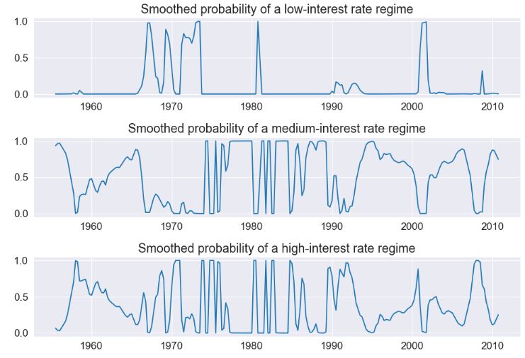
- Due to lower information criteria, we might prefer the 3-state model, with an interpretation of low-, medium-, and high-interest rate regimes. The smoothed probabilities of each regime are plotted below.
fig, axes = plt.subplots(3, figsize=(10, 7))

ax = axes[0]
ax.plot(res_fedfunds4.smoothed_marginal_probabilities[0])
ax.set(title="Smoothed probability of a low-interest rate regime")

ax = axes[1]
ax.plot(res_fedfunds4.smoothed_marginal_probabilities[1])
ax.set(title="Smoothed probability of a medium-interest rate regime")

ax = axes[2]
ax.plot(res_fedfunds4.smoothed_marginal_probabilities[2])
ax.set(title="Smoothed probability of a high-interest rate regime")

fig.tight_layout()
S&P 500 Absolute Returns
- Switching variances: We can also accommodate switching variances. The application is to absolute returns on S&P 500
from statsmodels.tsa.regime_switching.tests.test_markov_regression import areturns

dta_areturns = pd.Series(
    areturns, index=pd.date_range("2004-05-04", "2014-5-03", freq="W")
)

# Plot the data
dta_areturns.plot(title="Absolute returns, S&P500", figsize=(12, 3))

# Fit the model
mod_areturns = sm.tsa.MarkovRegression(
    dta_areturns.iloc[1:],
    k_regimes=2,
    exog=dta_areturns.iloc[:-1],
    switching_variance=True,
)
res_areturns = mod_areturns.fit()

res_areturns.summary()

Markov Switching Model Results
Dep. Variable:	y	No. Observations:	520
Model:	MarkovRegression	Log Likelihood	-745.798
Date:	Sat, 23 Dec 2023	AIC	1507.595
Time:	13:30:35	BIC	1541.626
Sample:	05-16-2004	HQIC	1520.926
- 04-27-2014
Covariance Type:	approx
Regime 0 parameters
coef	std err	z	P>|z|	[0.025	0.975]
const	0.7641	0.078	9.761	0.000	0.611	0.918
x1	0.0791	0.030	2.620	0.009	0.020	0.138
sigma2	0.3476	0.061	5.694	0.000	0.228	0.467
Regime 1 parameters
coef	std err	z	P>|z|	[0.025	0.975]
const	1.9728	0.278	7.086	0.000	1.427	2.518
x1	0.5280	0.086	6.155	0.000	0.360	0.696
sigma2	2.5771	0.405	6.357	0.000	1.783	3.372
Regime transition parameters
coef	std err	z	P>|z|	[0.025	0.975]
p[0->0]	0.7531	0.063	11.871	0.000	0.629	0.877
p[1->0]	0.6825	0.066	10.301	0.000	0.553	0.812
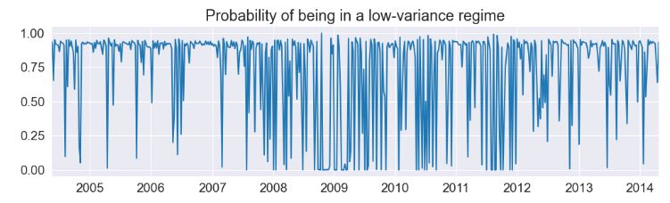
- The first regime is a low-variance regime and the second regime is a high-variance regime. Below we plot the probabilities of being in the low-variance regime. Between 2008 and 2012 there does not appear to be a clear indication of one regime guiding the economy.
res_areturns.smoothed_marginal_probabilities[0].plot(
    title="Probability of being in a low-variance regime", figsize=(12, 3)
)
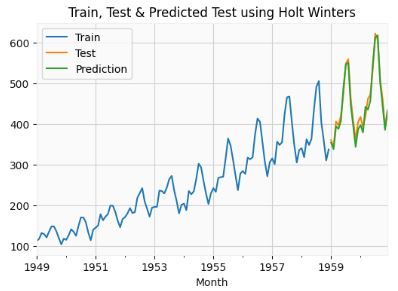
Number of Airline Passengers- 1. Holt-Winters
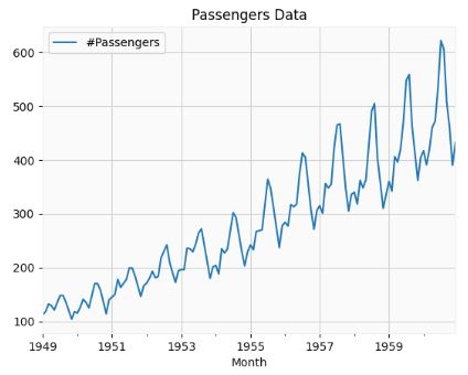
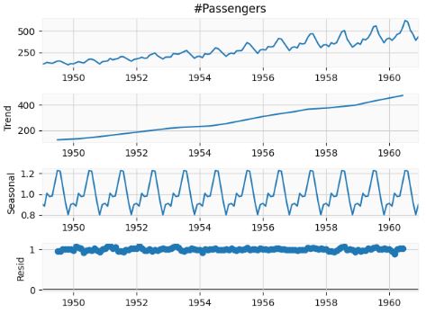
- Let’s apply the Holt-Winters Forecasting algorithm to the Airlines Passenger Data representing he number of International Airline Passengers (in thousands) between January 1949 to December 1960.
- Importing the key libraries and downloading the Kaggle dataset
# dataframe opertations - pandas
import pandas as pd
# plotting data - matplotlib
from matplotlib import pyplot as plt
# time series - statsmodels
# Seasonality decomposition
from statsmodels.tsa.seasonal import seasonal_decompose
from statsmodels.tsa.seasonal import seasonal_decompose
# holt winters
# single exponential smoothing
from statsmodels.tsa.holtwinters import SimpleExpSmoothing
# double and triple exponential smoothing
from statsmodels.tsa.holtwinters import ExponentialSmoothing
airline = pd.read_csv('AirPassengers.csv',index_col='Month', parse_dates=True)
# finding shape of the dataframe
print(airline.shape)
# having a look at the data
print(airline.head())
# plotting the original data
airline[['#Passengers']].plot(title='Passengers Data')
(144, 1)
            #Passengers
Month
1949-01-01          112
1949-02-01          118
1949-03-01          132
1949-04-01          129
1949-05-01          121
- Performing the seasonal decomposition of the input data
decompose_result = seasonal_decompose(airline['#Passengers'],model='multiplicative')
decompose_result.plot();
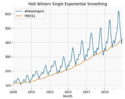
- Performing the Holt Winters (HW) Single Exponential Smoothing
# Set the frequency of the date time index as Monthly start as indicated by the data
airline.index.freq = 'MS'
# Set the value of Alpha and define m (Time Period)
m = 12
alpha = 1/(2*m)
airline['HWES1'] = SimpleExpSmoothing(airline['#Passengers']).fit(smoothing_level=alpha,optimized=False,use_brute=True).fittedvalues
airline[['#Passengers','HWES1']].plot(title='Holt Winters Single Exponential Smoothing');
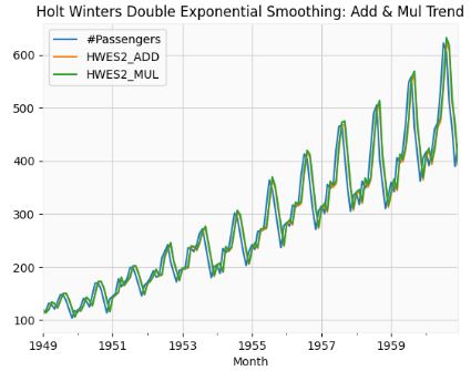
- Performing the HW Double Exponential Smoothing: Add & Mul Trend
airline['HWES2_ADD'] = ExponentialSmoothing(airline['#Passengers'],trend='add').fit().fittedvalues
airline['HWES2_MUL'] = ExponentialSmoothing(airline['#Passengers'],trend='mul').fit().fittedvalues
airline[['#Passengers','HWES2_ADD','HWES2_MUL']].plot(title='Holt Winters Double Exponential Smoothing: Add & Mul Trend');
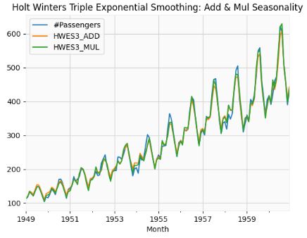
- Performing HW Triple Exponential Smoothing: Add & Mul Seasonality
airline['HWES3_ADD'] = ExponentialSmoothing(airline['#Passengers'],trend='add',seasonal='add',seasonal_periods=12).fit().fittedvalues
airline['HWES3_MUL'] = ExponentialSmoothing(airline['#Passengers'],trend='mul',seasonal='mul',seasonal_periods=12).fit().fittedvalues
airline[['#Passengers','HWES3_ADD','HWES3_MUL']].plot(title='Holt Winters Triple Exponential Smoothing: Add & Mul Seasonality');
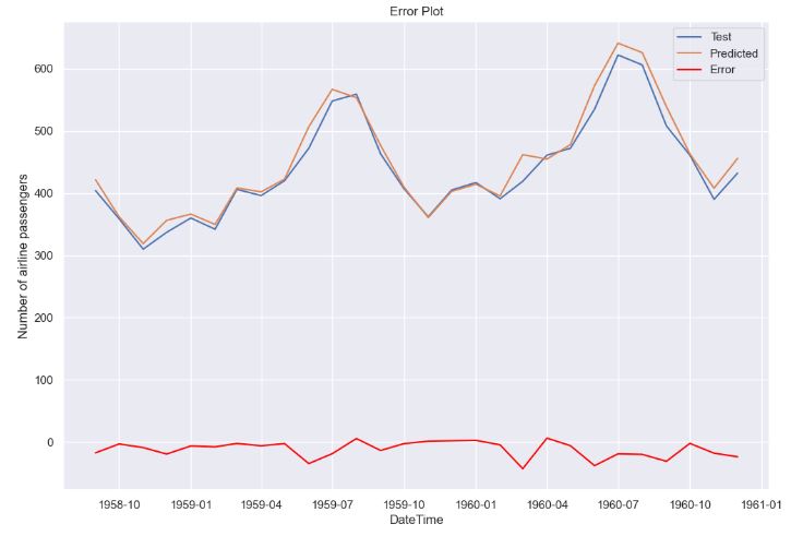
- Train, Test & Predicted Test using Holt Winters
# Split into train and test set
forecast_data=airline.copy()
train_airline = forecast_data[:120]
test_airline = forecast_data[120:]
fitted_model = ExponentialSmoothing(train_airline['#Passengers'],trend='mul',seasonal='mul',seasonal_periods=12).fit()
test_predictions = fitted_model.forecast(24)
train_airline['#Passengers'].plot(legend=True,label='Train')
test_airline['#Passengers'].plot(legend=True,label='Test',figsize=(6,4))
test_predictions.plot(legend=True,label='Prediction')
plt.title('Train, Test & Predicted Test using Holt Winters')
test_airline['#Passengers'].plot(legend=True,label='Test',figsize=(9,6))
test_predictions.plot(legend=True,label='Prediction',xlim=['1959–01–01','1961–01–01']);

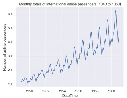
- Let’s apply the low-code open-source python framework pytsal to the Airlines Passenger Data
!git clone https://github.com/KrishnanSG/pytsal.git
cd pytsal
from pytsal.dataset import load_airline

ts = load_airline()

print(ts.summary())
print('\n### Data ###\n')
print(ts)
name             Monthly totals of international airline passen...
freq                                                            MS
target                                Number of airline passengers
type                                                    Univariate
phase                                                         Full
series_length                                                  144
start                                1949-01-01T00:00:00.000000000
end                                  1960-12-01T00:00:00.000000000
dtype: object

### Data ###

Date
1949-01-01    112.0
1949-02-01    118.0
1949-03-01    132.0
1949-04-01    129.0
1949-05-01    121.0
              ...
1960-08-01    606.0
1960-09-01    508.0
1960-10-01    461.0
1960-11-01    390.0
1960-12-01    432.0
Freq: MS, Name: Number of airline passengers, Length: 144, dtype: float64
- Performing the complete forecasting model setup & tuning
from pytsal.forecasting import *
model = setup(ts, 'holtwinter', eda=True, validation=True, find_best_model=True, plot_model_comparison=True)
INFO:pytsal.forecasting:Loading time series ...
INFO:pytsal.forecasting:Creating train test data
INFO:pytsal.forecasting:Initializing Visualizer ...
INFO:pytsal.visualization.eda:EDAVisualizer initialized
--- Time series summary ---

name             Monthly totals of international airline passen...
freq                                                            MS
target                                Number of airline passengers
type                                                    Univariate
phase                                                         Full
series_length                                                  144
start                                1949-01-01T00:00:00.000000000
end                                  1960-12-01T00:00:00.000000000
dtype: object
"Monthly totals of international airline passengers (1949 to 1960)" dataset split with train size: 116 test size: 28
INFO:pytsal.visualization.eda:Constructed Time plot
INFO:pytsal.visualization.eda:Constructed decompose plot
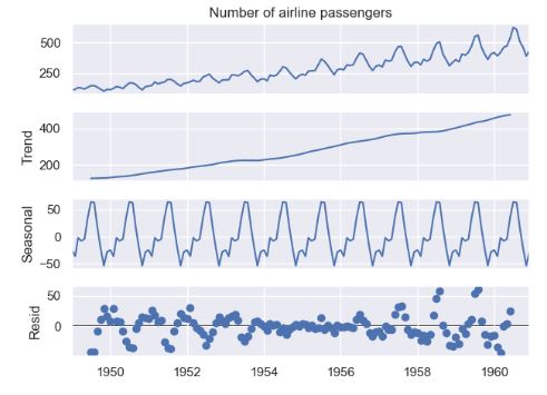
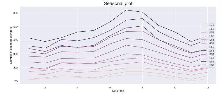
INFO:pytsal.visualization.eda:Constructed seasonal plot
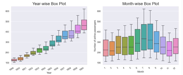
INFO:pytsal.visualization.eda:Constructed box plot
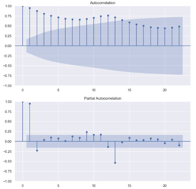
INFO:pytsal.visualization.eda:Constructed acf and pacf plot
INFO:pytsal.visualization.eda:Performing stationarity test
INFO:pytsal.visualization.eda:Test 1/2 ADF
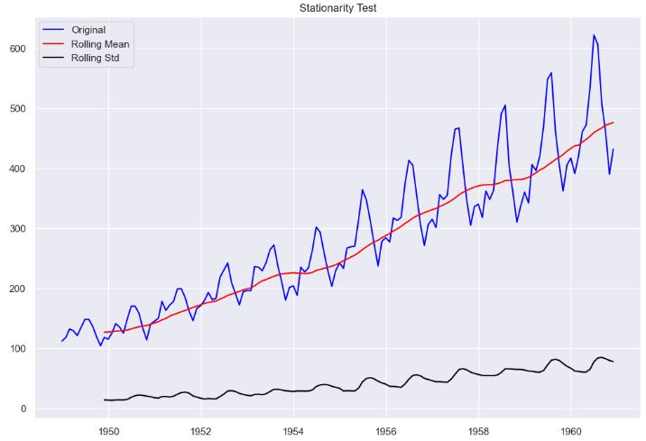
INFO:pytsal.visualization.eda:
Test 2/2 KPSS
INFO:pytsal.visualization.eda:Tests completed
INFO:pytsal.visualization.eda:Performed stationary tests
INFO:pytsal.visualization.eda:EDAVisualizer completed
INFO:pytsal.forecasting:Initialize model tuning ...
INFO:pytsal.forecasting:Initializing comparison plot ...
Results of Dickey-Fuller Test:
Test Statistic                   0.815369
p-value                          0.991880
#Lags Used                      13.000000
Number of Observations Used    130.000000
Critical Value 1%               -3.481682
Critical Value 5%               -2.884042
Critical Value 10%              -2.578770
dtype: float64
KPSS Statistic: 0.09614984853532524
p-value: 0.1
num lags: 4
Critial Values:
   10% : 0.119
   5% : 0.146
   2.5% : 0.176
   1% : 0.216

ADF: p-value = 0.9919. The series is likely non-stationary.
KPSS: The series is deterministic trend stationary
9 tunable params available for <class 'pytsal.internal.containers.models.forecasting.HoltWinter'>

INFO:pytsal.forecasting:Tuning completed
###### TUNING SUMMARY #####

   model_name                                 args       score    aicc
8  HoltWinter  {'trend': 'mul', 'seasonal': 'mul'}   13.053969  559.88
7  HoltWinter  {'trend': 'mul', 'seasonal': 'add'}   15.790874  607.52
6  HoltWinter  {'trend': 'add', 'seasonal': 'mul'}   20.691400  561.14
5  HoltWinter  {'trend': 'add', 'seasonal': 'add'}   23.616991  608.54
4  HoltWinter   {'trend': None, 'seasonal': 'mul'}   42.557011  509.11
2  HoltWinter   {'trend': None, 'seasonal': 'add'}   52.697958  635.81
0  HoltWinter    {'trend': None, 'seasonal': None}   91.816338  766.94
1  HoltWinter   {'trend': 'add', 'seasonal': None}  121.201352  769.53
3  HoltWinter   {'trend': 'mul', 'seasonal': None}  159.346430  770.16

Best model: {'trend': 'mul', 'seasonal': 'mul'} with score: 13.053969239269817
--- Model Summary ---
{'trend': 'mul', 'seasonal': 'mul'}

MAE      13.053969
MAPE      0.029033
RMSE     17.573640
AIC     552.826631
BIC     596.884074
AICC    559.878177
Name: Model metrics, dtype: float64
trained_model = finalize(ts, model)
INFO:pytsal.forecasting:Finalizing model (Training on complete data) ...

 ExponentialSmoothing Model Results
========================================================================================
Dep. Variable:     Number of airline passengers   No. Observations:                  144
Model:                     ExponentialSmoothing   SSE                          15805.297
Optimized:                                 True   AIC                            708.553
Trend:                           Multiplicative   BIC                            756.070
Seasonal:                        Multiplicative   AICC                           714.025
Seasonal Periods:                            12   Date:                 Tue, 02 Jan 2024
Box-Cox:                                  False   Time:                         18:06:56
Box-Cox Coeff.:                            None
=================================================================================
                          coeff                 code              optimized
---------------------------------------------------------------------------------
smoothing_level               0.2919245                alpha                 True
smoothing_trend              2.4068e-10                 beta                 True
smoothing_seasonal            0.5678907                gamma                 True
initial_level                 116.27509                  l.0                 True
initial_trend                 1.0091534                  b.0                 True
initial_seasons.0             0.9510089                  s.0                 True
initial_seasons.1             1.0025536                  s.1                 True
initial_seasons.2             1.1168827                  s.2                 True
initial_seasons.3             1.0647580                  s.3                 True
initial_seasons.4             0.9955442                  s.4                 True
initial_seasons.5             1.0918944                  s.5                 True
initial_seasons.6             1.1934906                  s.6                 True
initial_seasons.7             1.1805039                  s.7                 True
initial_seasons.8             1.0707840                  s.8                 True
initial_seasons.9             0.9271625                  s.9                 True
initial_seasons.10            0.8131458                 s.10                 True
initial_seasons.11            0.9419461                 s.11                 True
---------------------------------------------------------------------------------

save_model(trained_model)
INFO:pytsal.forecasting:Model saved to trained_model.pytsal
'Model saved'
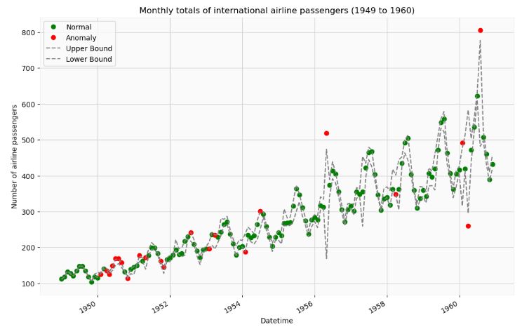
- The following example illustrates how the pytsal Holt-Winter’s model and the brutlag algorithm can be used to identify anomalies present in the above data.
import pytsal.forecasting as f
import pytsal.anomaly as ad

from pytsal.dataset import load_airline_with_anomaly

#1. Load data

ts_with_anomaly = load_airline_with_anomaly()

#print(ts_with_anomaly.summary())
#print('\n### Data ###\n')
#print(ts)

# 2.a Load model if exists
model = f.load_model()

# 2.b Create new model
if model is None:
    ts = load_airline()
    model = f.setup(ts, 'holtwinter', eda=False, validation=False, find_best_model=True, plot_model_comparison=False)
    trained_model = f.finalize(ts, model)
    f.save_model(trained_model)
    model = f.load_model()

# 3. brutlag algorithm finds and returns the anomaly points
anomaly_points = ad.setup(ts_with_anomaly, model, 'brutlag')

INFO:pytsal.forecasting:Model loaded from trained_model.pytsal
INFO:pytsal.anomaly:Initializing anomaly detection algorithm ...
WARNING:pytsal.anomaly:This function in future release will be refactored. Hence use this with care expecting breaking changes in upcoming versions.
INFO:pytsal.anomaly:Performing brutlag anomaly detection ...
Difference between actual and predicted

            actual   predicted  difference          UB          LB
Date
1949-01-01   112.0  111.590815    0.409185  111.892320  111.289311
1949-02-01   118.0  118.842908   -0.842908  119.463998  118.221818
1949-03-01   132.0  133.330735   -1.330735  134.311276  132.350193
1949-04-01   129.0  127.897958    1.102042  128.709989  127.085926
1949-05-01   121.0  120.982190    0.017810  120.995313  120.969068
...            ...         ...         ...         ...         ...
1960-08-01   806.0  629.399412  176.600588  777.057362  481.741463
1960-09-01   508.0  511.998458   -3.998458  526.868422  497.128493
1960-10-01   461.0  448.033463   12.966537  461.492241  434.574685
1960-11-01   390.0  397.251316   -7.251316  410.319061  384.183570
1960-12-01   432.0  437.148457   -5.148457  455.348078  418.948837

[144 rows x 5 columns]

The data points classified as anomaly

            observed    expected
date
1950-02-01     126.0  128.061306
1950-04-01     135.0  138.507945
1950-05-01     125.0  129.102592
1950-06-01     149.0  142.209534
1950-07-01     170.0  158.282617
1950-08-01     170.0  161.586634
1950-09-01     158.0  150.451460
1950-11-01     114.0  117.015788
1951-03-01     178.0  169.289921
1951-05-01     172.0  154.496337
1951-10-01     162.0  155.498759
1951-11-01     146.0  136.398227
1952-08-01     242.0  229.327484
1953-02-01     196.0  205.796078
1953-04-01     235.0  215.252036
1954-02-01     188.0  213.333317
1954-07-01     302.0  274.823045
1956-05-01     518.0  321.263814
1958-04-01     348.0  374.880420
1960-02-01     491.0  395.803036
1960-04-01     261.0  439.297376
1960-08-01     806.0  629.399412
Number of Airline Passengers- 2. Prophet
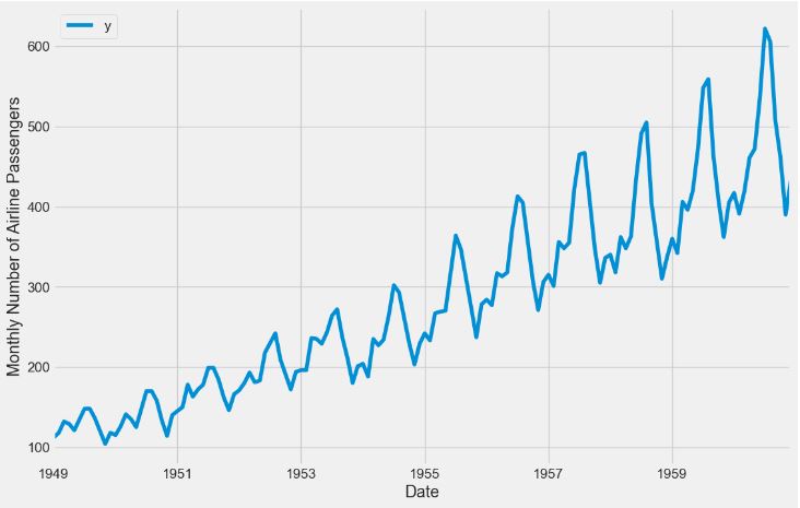
- In this section, we will apply the Prophet algorithm to the Airlines Passenger Data
- Preparing the input data
%matplotlib inline
import pandas as pd
from prophet import Prophet

import matplotlib.pyplot as plt
plt.style.use('fivethirtyeight')
df = pd.read_csv('AirPassengers.csv')
df['Month'] = pd.DatetimeIndex(df['Month'])
df = df.rename(columns={'Month': 'ds',
                        '#Passengers': 'y'})
ax = df.set_index('ds').plot(figsize=(12, 8))
ax.set_ylabel('Monthly Number of Airline Passengers')
ax.set_xlabel('Date')

plt.show()
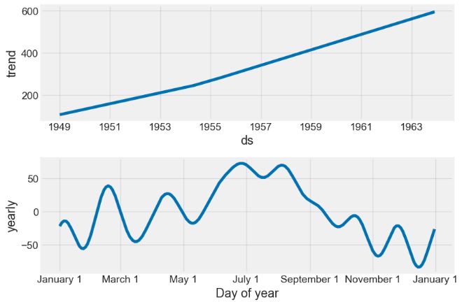
- Fitting the model and making predictions
# set the uncertainty interval to 95% (the Prophet default is 80%)
my_model = Prophet(interval_width=0.95)
my_model.fit(df)
future_dates = my_model.make_future_dataframe(periods=36, freq='MS')
future_dates.tail()
      ds
175	1963-08-01
176	1963-09-01
177	1963-10-01
178	1963-11-01
179	1963-12-01
forecast = my_model.predict(future_dates)
forecast[['ds', 'yhat', 'yhat_lower', 'yhat_upper']].tail()
my_model.plot(forecast,
              uncertainty=True)

my_model.plot_components(forecast)
Average Temperature in India
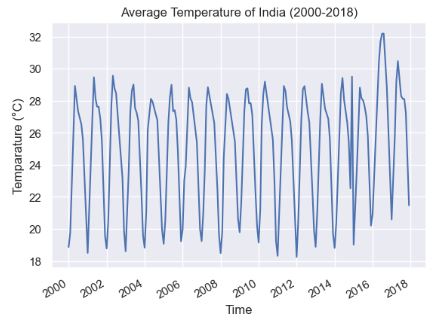
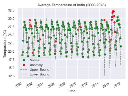
- Let’s apply the pytsal Holt-Winter’s model and the brutlag algorithm to the weather dataset that contains the India’s monthly average temperature (°C) from 2000-2018.
- Importing the input dataset
from time_series import TimeSeries

# Imports for data visualization
import matplotlib.pyplot as plt
import pandas as pd
from matplotlib.dates import DateFormatter
from matplotlib import dates as mpld

from pandas.plotting import register_matplotlib_converters
register_matplotlib_converters()

ts = TimeSeries('average_temp_india.csv', train_size=0.7)

plt.plot(ts.data.iloc[:,1].index,ts.data.iloc[:,1])
plt.gcf().autofmt_xdate()
plt.title("Average Temperature of India (2000-2018)")
plt.xlabel("Time")
plt.ylabel("Temparature (°C)")
plt.show()
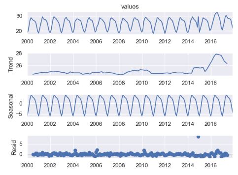
- Performing the additive seasonal decomposition of the above data
from statsmodels.tsa.seasonal import seasonal_decompose

seasonal_decompose(ts.data.iloc[:,1],model='additive',period=12).plot()
plt.show()
- Applying the anomaly detection algorithm to the temperature data
from time_series import TimeSeries

# Holt-Winters or Triple Exponential Smoothing model
from statsmodels.tsa.holtwinters import ExponentialSmoothing

# Imports for data visualization
import matplotlib.pyplot as plt
import pandas as pd
from matplotlib.dates import DateFormatter
from matplotlib import dates as mpld

from pandas.plotting import register_matplotlib_converters
register_matplotlib_converters()

ts = TimeSeries('average_temp_india.csv', train_size=0.7)

plt.plot(ts.data.iloc[:,1].index,ts.data.iloc[:,1])
plt.gcf().autofmt_xdate()
plt.title("Average Temperature of India (2000-2018)")
plt.xlabel("Time")
plt.ylabel("Temparature (°C)")
plt.show()

model = ExponentialSmoothing(
    ts.train, trend='additive', seasonal='additive').fit()
prediction = model.predict(
    start=ts.data.iloc[:, 1].index[0], end=ts.data.iloc[:, 1].index[-1])

"""Brutlag Algorithm"""
PERIOD = 12        # The given time series has seasonal_period=12
GAMMA = 0.3684211  # the seasonility component
SF = 1.96          # brutlag scaling factor for the confidence bands.
UB = []            # upper bound or upper confidence band
LB = []            # lower bound or lower confidence band

difference_array = []
dt = []
difference_table = {
    "actual": ts.data.iloc[:, 1], "predicted": prediction, "difference": difference_array, "UB": UB, "LB": LB}

"""Calculatation of confidence bands using brutlag algorithm"""
for i in range(len(prediction)):
    diff = ts.data.iloc[:, 1][i]-prediction[i]
    if i < PERIOD:
        dt.append(GAMMA*abs(diff))
    else:
        dt.append(GAMMA*abs(diff) + (1-GAMMA)*dt[i-PERIOD])

    difference_array.append(diff)
    UB.append(prediction[i]+SF*dt[i])
    LB.append(prediction[i]-SF*dt[i])

print("\nDifference between actual and predicted\n")
difference = pd.DataFrame(difference_table)
print(difference)

"""Classification of data points as either normal or anomaly"""
normal = []
normal_date = []
anomaly = []
anomaly_date = []

for i in range(len(ts.data.iloc[:, 1].index)):
    if (UB[i] <= ts.data.iloc[:, 1][i] or LB[i] >= ts.data.iloc[:, 1][i]) and i > PERIOD:
        anomaly_date.append(ts.data.index[i])
        anomaly.append(ts.data.iloc[:, 1][i])
    else:
        normal_date.append(ts.data.index[i])
        normal.append(ts.data.iloc[:, 1][i])

anomaly = pd.DataFrame({"date": anomaly_date, "value": anomaly})
anomaly.set_index('date', inplace=True)
normal = pd.DataFrame({"date": normal_date, "value": normal})
normal.set_index('date', inplace=True)

print("\nThe data points classified as anomaly\n")
print(anomaly)

Difference between actual and predicted

            actual  predicted  difference         UB         LB
2000-01-01   18.87  18.647206    0.222794  18.808087  18.486326
2000-02-01   19.78  20.668918   -0.888918  21.310810  20.027025
2000-03-01   23.22  24.025243   -0.805243  24.606713  23.443773
2000-04-01   27.27  26.716709    0.553291  27.116243  26.317175
2000-05-01   28.92  28.440959    0.479041  28.786877  28.095041
...            ...        ...         ...        ...        ...
2017-08-01   28.12  27.387160    0.732840  30.254620  24.519699
2017-09-01   28.11  26.760501    1.349499  29.704445  23.816557
2017-10-01   27.24  25.312988    1.927012  28.594966  22.031011
2017-11-01   23.92  22.620502    1.299498  25.266893  19.974111
2017-12-01   21.47  19.868828    1.601172  23.898407  15.839248

[216 rows x 5 columns]

The data points classified as anomaly

            value
date
2001-05-01  29.46
2001-06-01  28.13
2001-07-01  27.63
2001-08-01  27.62
2001-12-01  19.55
2002-07-01  28.47
2003-03-01  23.62
2006-01-01  19.96
2006-02-01  23.02
2008-12-01  20.62
2010-03-01  26.53
2010-07-01  27.55
2014-12-01  29.50
2016-01-01  20.92
2016-02-01  23.58
2016-04-01  29.56
2016-05-01  30.41
2016-06-01  31.70
2016-07-01  32.18
2016-08-01  32.19
2016-09-01  30.72
2016-10-01  28.81
2016-11-01  25.90

"""
Plotting the data points after classification as anomaly/normal.
Data points classified as anomaly are represented in red and normal in green.
"""
plt.plot(normal.index, normal, 'o', color='green')
plt.plot(anomaly.index, anomaly, 'o', color='red')

# Ploting brutlag confidence bands
plt.plot(ts.data.iloc[:, 1].index, UB, linestyle='--', color='grey')
plt.plot(ts.data.iloc[:, 1].index, LB, linestyle='--', color='grey')

# Formatting the graph
plt.legend(['Normal', 'Anomaly', 'Upper Bound', 'Lower Bound'])
plt.gcf().autofmt_xdate()
plt.title("Average Temperature of India (2000-2018)")
plt.xlabel("Time")
plt.ylabel("Temparature (°C)")
plt.show()
Monthly Sales Data Analysis
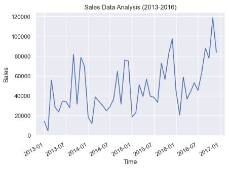
- Let’s apply the pytsal Holt-Winter’s model to the monthly total sales of a company from 2013-2016.
- Importing the input dataset
from time_series import TimeSeries

# Imports for data visualization
import matplotlib.pyplot as plt
from pandas.plotting import register_matplotlib_converters
from matplotlib.dates import DateFormatter
from matplotlib import dates as mpld

register_matplotlib_converters()

ts = TimeSeries('monthly_sales.csv', train_size=0.8)

print("Sales Data")
print(ts.data.describe())

print("Head and Tail of the time series")
print(ts.data.head(5).iloc[:,1])
print(ts.data.tail(5).iloc[:,1])

# Plot of raw time series data
plt.plot(ts.data.index,ts.data.sales)
plt.gcf().autofmt_xdate()
date_format = mpld.DateFormatter('%Y-%m')
plt.gca().xaxis.set_major_formatter(date_format)
plt.title("Sales Data Analysis (2013-2016)")
plt.xlabel("Time")
plt.ylabel("Sales")
plt.show()

Sales Data
               sales
count      48.000000
mean    47858.351667
std     25221.124187
min      4519.890000
25%     29790.100000
50%     39339.515000
75%     65833.345000
max    118447.830000
Head and Tail of the time series
date
2013-01-01    14236.90
2013-02-01     4519.89
2013-03-01    55691.01
2013-04-01    28295.35
2013-05-01    23648.29
Name: sales, dtype: float64
date
2016-08-01     63120.89
2016-09-01     87866.65
2016-10-01     77776.92
2016-11-01    118447.83
2016-12-01     83829.32
Name: sales, dtype: float64
- Performing the seasonal decomposition of the above data
from statsmodels.tsa.seasonal import seasonal_decompose

result_add = seasonal_decompose(ts.data.iloc[:,1],period=12,model='additive')
result_add.plot()
plt.gcf().autofmt_xdate()
date_format = mpld.DateFormatter('%y-%m')
plt.gca().xaxis.set_major_formatter(date_format)

result_mul = seasonal_decompose(ts.data.iloc[:,1],period=12,model='multiplicative')
result_mul.plot()
plt.gcf().autofmt_xdate()
date_format = mpld.DateFormatter('%y-%m')
plt.gca().xaxis.set_major_formatter(date_format)
plt.show()
- model=’additive’
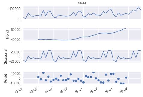
- model=’multiplicative’

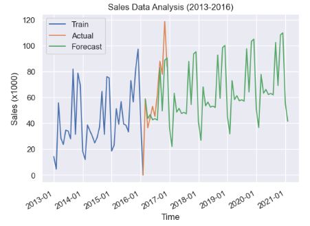
- Predicting the sales data with the Holt-Winter’s model
from statsmodels.tsa.holtwinters import ExponentialSmoothing
# Scaling down the data by a factor of 1000
ts.set_scale(1000)

# Training the model
model = ExponentialSmoothing(ts.train,trend='additive',seasonal='additive',seasonal_periods=12).fit(damping_slope=1)
plt.plot(ts.train.index,ts.train,label="Train")
plt.plot(ts.test.index,ts.test,label="Actual")

# Create a 5 year forecast
plt.plot(model.forecast(60),label="Forecast")

plt.legend(['Train','Actual','Forecast'])
plt.gcf().autofmt_xdate()
date_format = mpld.DateFormatter('%Y-%m')
plt.gca().xaxis.set_major_formatter(date_format)
plt.title("Sales Data Analysis (2013-2016)")
plt.xlabel("Time")
plt.ylabel("Sales (x1000)")
plt.show()
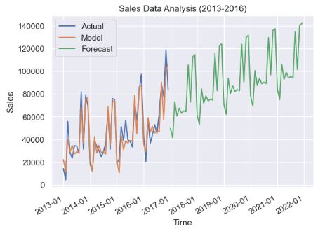
- Backtesting the training data with the additive and multiplicative Holt-Winter’s (HW) models
from statsmodels.tsa.holtwinters import ExponentialSmoothing
ts = TimeSeries('monthly_sales.csv', train_size=0.8)
# Additive model
model_add = ExponentialSmoothing(ts.data.iloc[:,1],trend='additive',seasonal='additive',seasonal_periods=12,damped=True).fit(damping_slope=0.98)
prediction = model_add.predict(start=ts.data.iloc[:,1].index[0],end=ts.data.iloc[:,1].index[-1])
plt.plot(ts.data.iloc[:,1].index,ts.data.iloc[:,1],label="Train")
plt.plot(ts.data.iloc[:,1].index,prediction,label="Model")
plt.plot(model_add.forecast(60))
plt.legend(['Actual','Model','Forecast'])
plt.gcf().autofmt_xdate()
date_format = mpld.DateFormatter('%Y-%m')
plt.gca().xaxis.set_major_formatter(date_format)
plt.title("Sales Data Analysis (2013-2016)")
plt.xlabel("Time")
plt.ylabel("Sales")
plt.show()
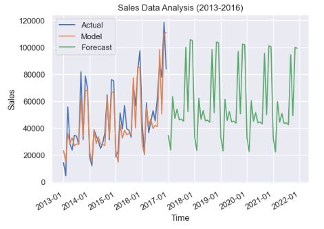
# Multiplicative model
model_mul = ExponentialSmoothing(ts.data.iloc[:,1],trend='additive',seasonal='multiplicative',seasonal_periods=12,damped=True).fit()
prediction = model_mul.predict(start=ts.data.iloc[:,1].index[0],end=ts.data.iloc[:,1].index[-1])
plt.plot(ts.data.iloc[:,1].index,ts.data.iloc[:,1],label="Train")
plt.plot(ts.data.iloc[:,1].index,prediction,label="Model")
plt.plot(model_mul.forecast(60))
plt.legend(['Actual','Model','Forecast'])
plt.gcf().autofmt_xdate()
date_format = mpld.DateFormatter('%Y-%m')
plt.gca().xaxis.set_major_formatter(date_format)
plt.title("Sales Data Analysis (2013-2016)")
plt.xlabel("Time")
plt.ylabel("Sales")
plt.show()
- Additive HW model
- Multiplicative HW model
- Printing the HW model summary
print(model_add.summary())

ExponentialSmoothing Model Results
================================================================================
Dep. Variable:                    sales   No. Observations:                   48
Model:             ExponentialSmoothing   SSE                     3839988196.858
Optimized:                         True   AIC                            907.482
Trend:                         Additive   BIC                            939.292
Seasonal:                      Additive   AICC                           934.624
Seasonal Periods:                    12   Date:                 Sun, 10 Dec 2023
Box-Cox:                          False   Time:                         16:00:40
Box-Cox Coeff.:                    None
=================================================================================
                          coeff                 code              optimized
---------------------------------------------------------------------------------
smoothing_level               0.1464286                alpha                 True
smoothing_trend               0.1464286                 beta                 True
smoothing_seasonal               0.0001                gamma                 True
initial_level                 41082.694                  l.0                 True
initial_trend                -156.87900                  b.0                 True
damping_trend                 0.9800000                  phi                False
initial_seasons.0            -18766.692                  s.0                 True
initial_seasons.1            -28179.421                  s.1                 True
initial_seasons.2             2468.4814                  s.2                 True
initial_seasons.3            -11199.301                  s.3                 True
initial_seasons.4            -5356.2134                  s.4                 True
initial_seasons.5            -10732.448                  s.5                 True
initial_seasons.6            -9770.2038                  s.6                 True
initial_seasons.7            -11438.903                  s.7                 True
initial_seasons.8             28700.401                  s.8                 True
initial_seasons.9            -4778.0170                  s.9                 True
initial_seasons.10            33978.828                 s.10                 True
initial_seasons.11            35073.489                 s.11                 True
---------------------------------------------------------------------------------

print(model_mul.summary())
ExponentialSmoothing Model Results
================================================================================
Dep. Variable:                    sales   No. Observations:                   48
Model:             ExponentialSmoothing   SSE                     5306329076.722
Optimized:                         True   AIC                            923.006
Trend:                         Additive   BIC                            954.817
Seasonal:                Multiplicative   AICC                           950.149
Seasonal Periods:                    12   Date:                 Sun, 10 Dec 2023
Box-Cox:                          False   Time:                         16:00:40
Box-Cox Coeff.:                    None
=================================================================================
                          coeff                 code              optimized
---------------------------------------------------------------------------------
smoothing_level               0.1464286                alpha                 True
smoothing_trend                  0.0001                 beta                 True
smoothing_seasonal               0.0001                gamma                 True
initial_level                 41082.694                  l.0                 True
initial_trend                -158.47980                  b.0                 True
damping_trend                 0.9900000                  phi                 True
initial_seasons.0             0.5674311                  s.0                 True
initial_seasons.1             0.3899121                  s.1                 True
initial_seasons.2             1.0435695                  s.2                 True
initial_seasons.3             0.7787636                  s.3                 True
initial_seasons.4             0.8913974                  s.4                 True
initial_seasons.5             0.7633235                  s.5                 True
initial_seasons.6             0.7722301                  s.6                 True
initial_seasons.7             0.7479818                  s.7                 True
initial_seasons.8             1.6619738                  s.8                 True
initial_seasons.9             0.8691594                  s.9                 True
initial_seasons.10            1.7613772                 s.10                 True
initial_seasons.11            1.7528805                 s.11                 True
---------------------------------------------------------------------------------
- One can see that IC(model_add)<IC(model_mul), where IC=AIC, BIC, and AICC. Recall that the smaller the IC value, the better the model fit.
"""
Conclusion of the analysis
--------------------------
From the model summary obtained it is clear that the sum of squared errors (SSE) for
the additive model (5088109579.122) < the SSE for the multiplicative(5235252441.242) model.

Hence the initial assumption that seasonality is roughly constant and therefore choosing
additive model was appropriate.

Note: The forecast made using multiplicative model seems to be unrealistic since the
variance between the high and low on an average is 100000 which is somewhat unexpected in
real world sales compared to 63000 incase of additive model.
"""
QC Audit of Rossmann Stores
- Let’s look at the Rossmann Store Sales representing historical sales data for 1,115 Rossmann stores. Our ultimate goal is to forecast the “Sales” column for the test set. Data challenge: some stores in the dataset were temporarily closed for refurbishment.
- Importing the key libraries
import warnings
warnings.filterwarnings("ignore")

# loading packages
# basic + dates
import numpy as np
import pandas as pd
from pandas import datetime

# data visualization
import matplotlib.pyplot as plt
import seaborn as sns # advanced vizs
%matplotlib inline

# statistics
#https://towardsdatascience.com/what-why-and-how-to-read-empirical-cdf-123e2b922480
from statsmodels.distributions.empirical_distribution import ECDF

# time series analysis
from statsmodels.tsa.seasonal import seasonal_decompose
from statsmodels.graphics.tsaplots import plot_acf, plot_pacf

# prophet by Facebook
from prophet import Prophet
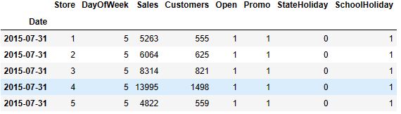
- Importing the train set and additional store data
# importing train data to learn
train = pd.read_csv("train.csv",
                    parse_dates = True, low_memory = False, index_col = 'Date')

# additional store data
store = pd.read_csv("store.csv",
                    low_memory = False)
# time series as indexes
train.index

DatetimeIndex(['2015-07-31', '2015-07-31', '2015-07-31', '2015-07-31',
               '2015-07-31', '2015-07-31', '2015-07-31', '2015-07-31',
               '2015-07-31', '2015-07-31',
               ...
               '2013-01-01', '2013-01-01', '2013-01-01', '2013-01-01',
               '2013-01-01', '2013-01-01', '2013-01-01', '2013-01-01',
               '2013-01-01', '2013-01-01'],
              dtype='datetime64[ns]', name='Date', length=1017209, freq=None)
print(train.shape)
train.head()
(1017209, 8)
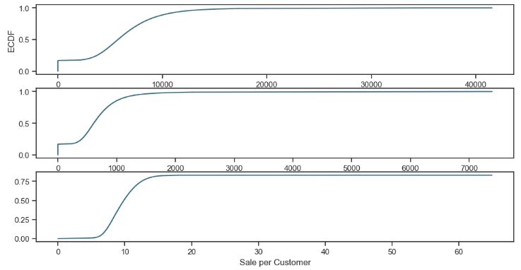
- Data editing, descriptive statistics, and plotting ECDF
# data extraction
train['Year'] = train.index.year
train['Month'] = train.index.month
train['Day'] = train.index.day
train['WeekOfYear'] = train.index.weekofyear

# adding new variable
train['SalePerCustomer'] = train['Sales']/train['Customers']
train['SalePerCustomer'].describe()
count    844340.000000
mean          9.493619
std           2.197494
min           0.000000
25%           7.895563
50%           9.250000
75%          10.899729
max          64.957854
Name: SalePerCustomer, dtype: float64

sns.set(style = "ticks")# to format into seaborn
c = '#386B7F' # basic color for plots
plt.figure(figsize = (12, 6))

plt.subplot(311)
cdf = ECDF(train['Sales'])
plt.plot(cdf.x, cdf.y, label = "statmodels", color = c);
plt.xlabel('Sales'); plt.ylabel('ECDF');

# plot second ECDF
plt.subplot(312)
cdf = ECDF(train['Customers'])
plt.plot(cdf.x, cdf.y, label = "statmodels", color = c);
plt.xlabel('Customers');

# plot second ECDF
plt.subplot(313)
cdf = ECDF(train['SalePerCustomer'])
plt.plot(cdf.x, cdf.y, label = "statmodels", color = c);
plt.xlabel('Sale per Customer');
- Checking open stores with zero sales
train[(train.Open==0)].shape
(172817, 13)
# opened stores with zero sales
zero_sales = train[(train.Open != 0) & (train.Sales == 0)]
print("In total: ", zero_sales.shape)
#zero_sales.head(5)
In total:  (54, 13)
- Closed stores and days which didn’t have any sales won’t be counted into the forecasts
print("Closed stores and days which didn't have any sales won't be counted into the forecasts.")
train = train[(train["Open"] != 0) & (train['Sales'] != 0)]

print("In total: ", train.shape)
Closed stores and days which didn't have any sales won't be counted into the forecasts.
In total:  (844338, 13)
- Checking missing values
#missing values
store.isnull().sum()
Store                          0
StoreType                      0
Assortment                     0
CompetitionDistance            3
CompetitionOpenSinceMonth    354
CompetitionOpenSinceYear     354
Promo2                         0
Promo2SinceWeek              544
Promo2SinceYear              544
PromoInterval                544
dtype: int64
- Dealing with NaN values
# fill NaN with a median value (skewed distribuion)
store['CompetitionDistance'].fillna(store['CompetitionDistance'].median(), inplace = True)
# filling NAN value with zero
store.fillna(0, inplace = True)
- Merging train and additional store information
print("Joining train set with an additional store information.")

# by specifying inner join we make sure that only those observations
# that are present in both train and store sets are merged together
train_store = pd.merge(train, store, how = 'inner', on = 'Store')

print("In total: ", train_store.shape)
#train_store.head()
Joining train set with an additional store information.
In total:  (844338, 22)
- Creating 4 groups of stores for QC analysis
train_store.groupby('StoreType')['Customers', 'Sales'].sum()
	Customers	Sales
StoreType
a	363541431	3165334859
b	31465616	159231395
c	92129705	783221426
d	156904995	1765392943
- Monthly sales trends
# sales trends
sns.factorplot(data = train_store, x = 'Month', y = "Sales",
               palette = 'plasma',
               row = 'Promo',
               hue = 'StoreType',
               color = c)
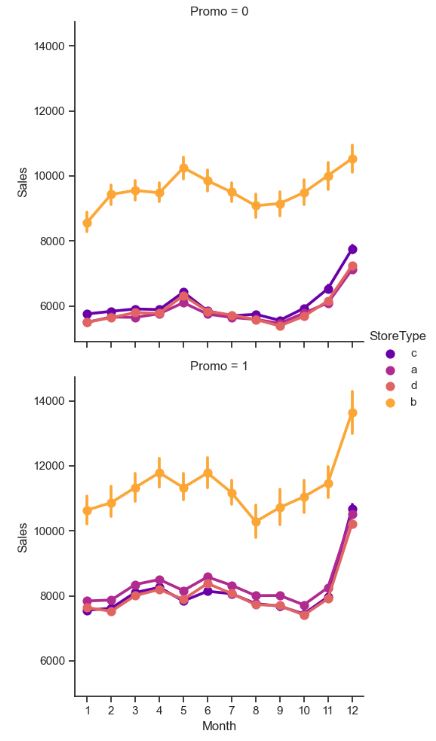
- Monthly trends customers
# sales trends
sns.factorplot(data = train_store, x = 'Month', y = "Customers",
               palette = 'plasma',
               col = 'Promo',
               hue = 'StoreType',
               color = c)

- Sale per customer trends
# sale per customer trends
sns.factorplot(data = train_store, x = 'Month', y = "SalePerCustomer",
               palette = 'plasma',
               hue = 'StoreType',
               col = 'Promo', # per promo in the store in rows
               color = c)
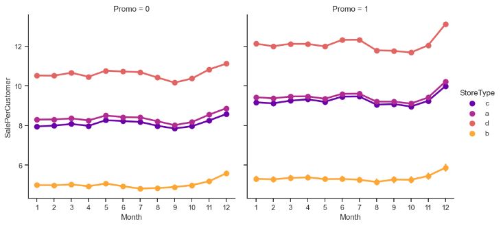
- Stores open on Sundays
# stores open on Sundays
train_store[(train_store.Open == 1) & (train_store.DayOfWeek == 7)]['Store'].unique()
array([  85,  122,  209,  259,  262,  274,  299,  310,  335,  353,  423,
        433,  453,  494,  512,  524,  530,  562,  578,  676,  682,  732,
        733,  769,  863,  867,  877,  931,  948, 1045, 1081, 1097, 1099],
      dtype=int64)
- Data editing
 #competition open time (in months)
train_store['CompetitionOpen'] = 12 * (train_store.Year - train_store.CompetitionOpenSinceYear) + (train_store.Month - train_store.CompetitionOpenSinceMonth)
# Promo open time
# to convert weeks into momths we divided by 4
train_store['PromoOpen'] = 12 * (train_store.Year - train_store.Promo2SinceYear) +(train_store.WeekOfYear - train_store.Promo2SinceWeek) / 4.0
# replace NA's by 0
train_store.fillna(0, inplace = True)
# average PromoOpen time and CompetitionOpen time per store type
train_store.loc[:, ['StoreType', 'Sales', 'Customers', 'PromoOpen', 'CompetitionOpen']].groupby('StoreType').mean()
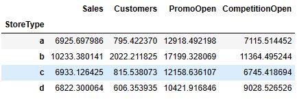
- Plotting the input data correlation matrix, excluding ‘Open’
import seaborn as sns
# Compute the correlation matrix
# exclude 'Open' variable
corr_all = train_store.drop('Open', axis = 1).corr()

 # Draw the heatmap with the mask and correct aspect ratio
sns.heatmap(corr_all, square = True, linewidths = .5, cmap = "BuPu")
plt.show()
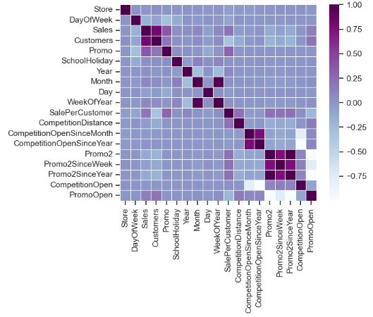
- Sales vs days of the week
sns.factorplot(data = train_store, x = 'DayOfWeek', y = "Sales",
               col = 'Promo',
               hue = 'Promo2',
               palette = 'copper_r')

Rossmann Sales Forecasting – 1. Prophet
- Preparing the Rossmann sales data for Prophet TSF
#prophet
# importing data
df = pd.read_csv("train.csv")
# remove closed stores and those with no sales
df = df[(df["Open"] != 0) & (df['Sales'] != 0)]

# sales for the store number 1 (StoreType C)
sales = df[df.Store == 1].loc[:, ['Date', 'Sales']]

# reverse to the order: from 2013 to 2015
sales = sales.sort_index(ascending = False)

# to datetime64
sales['Date'] = pd.DatetimeIndex(sales['Date'])
sales.dtypes
Date     datetime64[ns]
Sales             int64
dtype: object
# from the prophet documentation every variables should have specific names
sales = sales.rename(columns = {'Date': 'ds',
                                'Sales': 'y'})
sales.head()
              ds	y
1014980	2013-01-02	5530
1013865	2013-01-03	4327
1012750	2013-01-04	4486
1011635	2013-01-05	4997
1009405	2013-01-07	7176

# plot daily sales
ax = sales.set_index('ds').plot(figsize = (12, 4), color = c)
ax.set_ylabel('Daily Number of Sales')
ax.set_xlabel('Date')
plt.show()
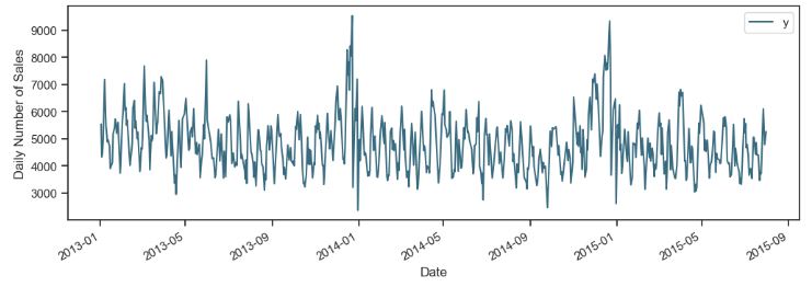
- Implementing the Prophet sales predictions
# set the uncertainty interval to 95% (the Prophet default is 80%)
my_model = Prophet(interval_width = 0.95)
my_model.fit(sales)

# dataframe that extends into future 6 weeks
future_dates = my_model.make_future_dataframe(periods = 6*7)

print("First week to forecast.")
future_dates.tail(7)

First week to forecast.
      ds
816	2015-09-05
817	2015-09-06
818	2015-09-07
819	2015-09-08
820	2015-09-09
821	2015-09-10
822	2015-09-11

# predictions
forecast = my_model.predict(future_dates)

# preditions for last week
forecast[['ds', 'yhat', 'yhat_lower', 'yhat_upper']].tail(7)

          ds	yhat	    yhat_lower	yhat_upper
816	2015-09-05	4292.409701	2653.425965	6050.839017
817	2015-09-06	4269.087297	2601.628302	6095.321680
818	2015-09-07	4490.506173	2820.014897	6138.015054
819	2015-09-08	3982.036581	2347.097300	5597.934327
820	2015-09-09	3849.129901	2087.806972	5470.880577
821	2015-09-10	3746.277635	2051.671578	5445.616615
822	2015-09-11	3990.467491	2281.187988	5753.217991

fc = forecast[['ds', 'yhat']].rename(columns = {'Date': 'ds', 'Forecast': 'yhat'})

# visualizing predicions
my_model.plot(forecast);
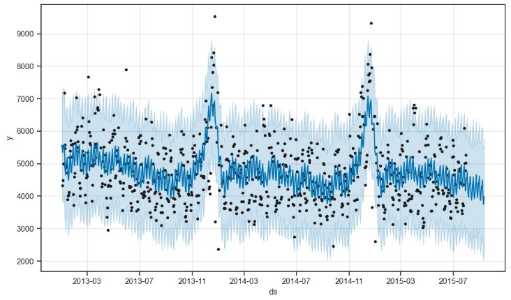
- Plotting the key components of the Prophet forecast
my_model.plot_components(forecast);
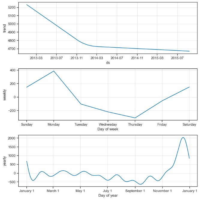
Rossmann Sales Forecasting – 2. SARIMA
- Preparing the Rossmann sales data for SARIMA TSF.
# additional store data
store = pd.read_csv("store.csv")
train = pd.read_csv("train.csv", parse_dates = True, low_memory = False, index_col = 'Date')

# data extraction, lets make new features about date time

train['Year'] = train.index.year
train['Month'] = train.index.month
train['Day'] = train.index.day
train['WeekOfYear'] = train.index.weekofyear

# adding new variable, no of sales per customer

train['SalePerCustomer'] = train['Sales']/train['Customers']

train.fillna(0, inplace = True)
# opened stores with zero sales
zero_sales = train[(train.Open != 0) & (train.Sales == 0)]
print("In total: ", zero_sales.shape)
In total:  (54, 13)
train = train[(train["Open"] != 0) & (train['Sales'] != 0)]

print("In total: ", train.shape)
In total:  (844338, 13)

train=train.drop(columns=train[(train.Open == 1) & (train.Sales == 0)].index)
store['CompetitionDistance'].fillna(store['CompetitionDistance'].median(), inplace = True)
# replace NA's by 0
store.fillna(0, inplace = True)
print("Joining train set with an additional store information.")

# by specifying inner join we make sure that only those observations
# that are present in both train and store sets are merged together in this data 'store' is present in both
train_store = pd.merge(train, store, how = 'inner', on = 'Store')

print("In total: ", train_store.shape)
Joining train set with an additional store information.
In total:  (844338, 22)

# competition open time (in months)
train_store['CompetitionOpen'] = 12 * (train_store.Year - train_store.CompetitionOpenSinceYear) + \
        (train_store.Month - train_store.CompetitionOpenSinceMonth)

# Promo open time
train_store['PromoOpen'] = 12 * (train_store.Year - train_store.Promo2SinceYear) + \
        (train_store.WeekOfYear - train_store.Promo2SinceWeek) / 4.0

# replace NA's by 0
train_store.fillna(0, inplace = True)

# average PromoOpen time and CompetitionOpen time per store type
train_store.loc[:, ['StoreType', 'Sales', 'Customers', 'PromoOpen', 'CompetitionOpen']].groupby('StoreType').mean()

       Sales	Customers	PromoOpen	CompetitionOpen
StoreType
a	6925.697986	795.422370	12918.492198	7115.514452
b	10233.380141	2022.211825	17199.328069	11364.495244
c	6933.126425	815.538073	12158.636107	6745.418694
d	6822.300064	606.353935	10421.916846	9028.526526

# HeatMap
# Compute the correlation matrix
# exclude 'Open' variable
corr_all = train_store.drop('Open', axis = 1).corr()

# Generate a mask for the upper triangle
mask = np.zeros_like(corr_all, dtype = np.bool)
mask[np.triu_indices_from(mask)] = True

# Set up the matplotlib figure
f, ax = plt.subplots(figsize = (11, 9))

# Draw the heatmap with the mask and correct aspect ratio
sns.heatmap(corr_all, mask = mask, annot = True, square = True, linewidths = 0.5, ax = ax, cmap = "BrBG", fmt='.2f')
plt.show()

- Creating 4 store types a, b, c, and d
# preparation: input should be float64 type
train['Sales'] = train['Sales'] * 1.0

# store types
sales_a = train[train.Store == 6]['Sales']
sales_b = train[train.Store == 75]['Sales']
sales_c = train[train.Store == 8]['Sales']
sales_d = train[train.Store == 26]['Sales']
- Plotting trends of 4 store types
f, (ax1, ax2, ax3, ax4) = plt.subplots(4, figsize = (12, 13))

# monthly
decomposition_a = seasonal_decompose(sales_a, model = 'additive', period = 365)
decomposition_a.trend.plot(color = c, ax = ax1)

decomposition_b = seasonal_decompose(sales_b, model = 'additive', period = 365)
decomposition_b.trend.plot(color = c, ax = ax2)

decomposition_c = seasonal_decompose(sales_c, model = 'additive', period = 365)
decomposition_c.trend.plot(color = c, ax = ax3)

decomposition_d = seasonal_decompose(sales_d, model = 'additive', period = 365)
decomposition_d.trend.plot(color = c, ax = ax4)
- Trends of 4 store types: a, b, c, and d (from top to bottom)
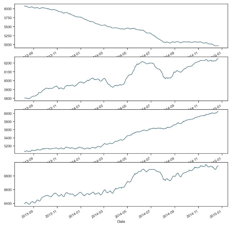
- Introducing the test stationarity and residual plot functions
from statsmodels.tsa.stattools import adfuller
def test_stationarity(timeseries, window = 12, cutoff = 0.01):

    #Determing rolling statistics
    rolmean = timeseries.rolling(window).mean()
    rolstd = timeseries.rolling(window).std()

    #Plot rolling statistics:
    fig = plt.figure(figsize=(12, 8))
    orig = plt.plot(timeseries, color='blue',label='Original')
    mean = plt.plot(rolmean, color='red', label='Rolling Mean')
    std = plt.plot(rolstd, color='black', label = 'Rolling Std')
    plt.legend(loc='best')
    plt.title('Rolling Mean & Standard Deviation')
    plt.show()

    #Perform Dickey-Fuller test:
    print('Results of Dickey-Fuller Test:')
    dftest = adfuller(timeseries, autolag='AIC', maxlag = 20 )
    dfoutput = pd.Series(dftest[0:4], index=['Test Statistic','p-value','#Lags Used','Number of Observations Used'])
    for key,value in dftest[4].items():
        dfoutput['Critical Value (%s)'%key] = value
    pvalue = dftest[1]
    if pvalue < cutoff:
        print('p-value = %.4f. The series is likely stationary.' % pvalue)
    else:
        print('p-value = %.4f. The series is likely non-stationary.' % pvalue)

    print(dfoutput)

from scipy import stats
from scipy.stats import normaltest
def residual_plot(model):

    resid = model.resid
    print(normaltest(resid))
    # returns a 2-tuple of the chi-squared statistic, and the associated p-value. the p-value is very small, meaning
    # the residual is not a normal distribution

    fig = plt.figure(figsize=(12,8))
    ax0 = fig.add_subplot(111)

    sns.distplot(resid ,fit = stats.norm, ax = ax0) # need to import scipy.stats

    # Get the fitted parameters used by the function
    (mu, sigma) = stats.norm.fit(resid)

    #Now plot the distribution using
    plt.legend(['Normal dist. ($\mu=$ {:.2f} and $\sigma=$ {:.2f} )'.format(mu, sigma)], loc='best')
    plt.ylabel('Frequency')
    plt.title('Residual distribution')


    # ACF and PACF
    fig = plt.figure(figsize=(12,8))
    ax1 = fig.add_subplot(211)
    fig = sm.graphics.tsa.plot_acf(model.resid, lags=40, ax=ax1)
    ax2 = fig.add_subplot(212)
    fig = sm.graphics.tsa.plot_pacf(model.resid, lags=40, ax=ax2)
- Test stationarity sales (a)
test_stationarity(sales_a)
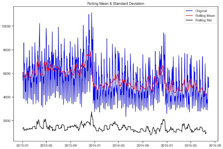
Results of Dickey-Fuller Test:
p-value = 0.0040. The series is likely stationary.
Test Statistic                  -3.710315
p-value                          0.003970
#Lags Used                      13.000000
Number of Observations Used    766.000000
Critical Value (1%)             -3.438916
Critical Value (5%)             -2.865321
Critical Value (10%)            -2.568783
dtype: float64
- Test stationarity sales (a) 1st difference
first_diff_a = sales_a - sales_a.shift(1)
first_diff_a = first_diff_a.dropna(inplace = False)
test_stationarity(first_diff_a, window = 12)
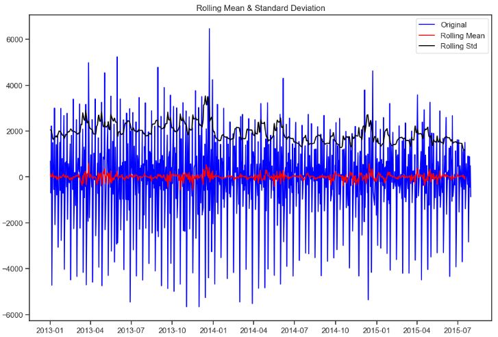
Results of Dickey-Fuller Test:
p-value = 0.0000. The series is likely stationary.
Test Statistic                -9.622589e+00
p-value                        1.693425e-16
#Lags Used                     2.000000e+01
Number of Observations Used    7.580000e+02
Critical Value (1%)           -3.439006e+00
Critical Value (5%)           -2.865361e+00
Critical Value (10%)          -2.568804e+00
dtype: float64
- Test stationarity sales (b)
test_stationarity(sales_b)
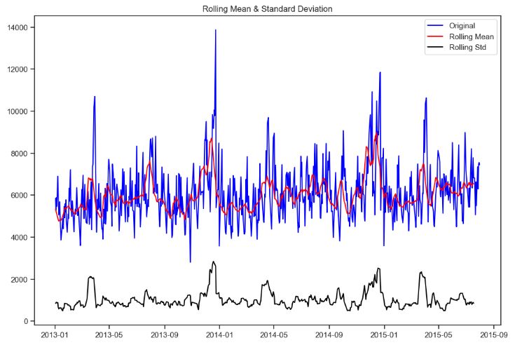
Results of Dickey-Fuller Test:
p-value = 0.0000. The series is likely stationary.
Test Statistic                  -5.056391
p-value                          0.000017
#Lags Used                      18.000000
Number of Observations Used    765.000000
Critical Value (1%)             -3.438927
Critical Value (5%)             -2.865325
Critical Value (10%)            -2.568786
- Test stationarity sales (b) 1st difference
first_diff_b = sales_b - sales_b.shift(1)
first_diff_b = first_diff_b.dropna(inplace = False)
test_stationarity(first_diff_b, window = 12)
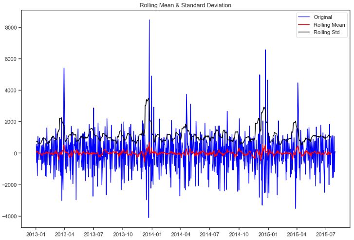
Results of Dickey-Fuller Test:
p-value = 0.0000. The series is likely stationary.
Test Statistic                -9.909451e+00
p-value                        3.197879e-17
#Lags Used                     2.000000e+01
Number of Observations Used    7.620000e+02
Critical Value (1%)           -3.438961e+00
Critical Value (5%)           -2.865340e+00
Critical Value (10%)          -2.568794e+00
- Test stationarity sales (c)
test_stationarity(sales_c)
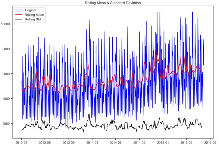
Results of Dickey-Fuller Test:
p-value = 0.0163. The series is likely non-stationary.
Test Statistic                  -3.268438
p-value                          0.016350
#Lags Used                      18.000000
Number of Observations Used    765.000000
Critical Value (1%)             -3.438927
Critical Value (5%)             -2.865325
Critical Value (10%)            -2.568786
dtype: float64
- Test stationarity sales (c) 1st difference
first_diff_c = sales_c - sales_c.shift(1)
first_diff_c = first_diff_c.dropna(inplace = False)
test_stationarity(first_diff_c, window = 12)
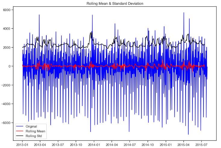
Results of Dickey-Fuller Test:
p-value = 0.0000. The series is likely stationary.
Test Statistic                -1.064255e+01
p-value                        4.887792e-19
#Lags Used                     2.000000e+01
Number of Observations Used    7.620000e+02
Critical Value (1%)           -3.438961e+00
Critical Value (5%)           -2.865340e+00
Critical Value (10%)          -2.568794e+00
dtype: float64
- Test stationarity sales (d)
test_stationarity(sales_d)
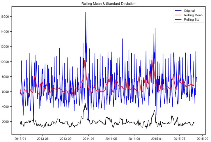
Results of Dickey-Fuller Test:
p-value = 0.0000. The series is likely stationary.
Test Statistic                -5.830805e+00
p-value                        3.979389e-07
#Lags Used                     1.500000e+01
Number of Observations Used    7.660000e+02
Critical Value (1%)           -3.438916e+00
Critical Value (5%)           -2.865321e+00
Critical Value (10%)          -2.568783e+00
dtype: float64
- Test stationarity sales (d) 1st difference
first_diff_d = sales_d - sales_d.shift(1)
first_diff_d = first_diff_d.dropna(inplace = False)
test_stationarity(first_diff_d, window = 12)
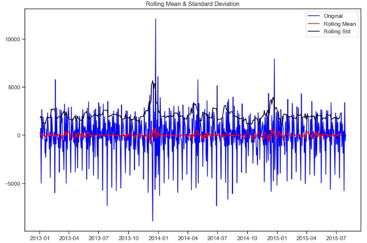
Results of Dickey-Fuller Test:
p-value = 0.0000. The series is likely stationary.
Test Statistic                -1.090009e+01
p-value                        1.165171e-19
#Lags Used                     1.600000e+01
Number of Observations Used    7.640000e+02
Critical Value (1%)           -3.438938e+00
Critical Value (5%)           -2.865330e+00
Critical Value (10%)          -2.568788e+00
dtype: float64
- Plotting ACF and PACF for 4 sales types: a, b, c, and d (from top to bottom)
# figure for subplots
plt.figure(figsize = (12, 8))

# acf and pacf for A
plt.subplot(421); plot_acf(sales_a, lags = 50, ax = plt.gca(), color = c)
plt.subplot(422); plot_pacf(sales_a, lags = 50, ax = plt.gca(), color = c)

# acf and pacf for B
plt.subplot(423); plot_acf(sales_b, lags = 50, ax = plt.gca(), color = c)
plt.subplot(424); plot_pacf(sales_b, lags = 50, ax = plt.gca(), color = c)

# acf and pacf for C
plt.subplot(425); plot_acf(sales_c, lags = 50, ax = plt.gca(), color = c)
plt.subplot(426); plot_pacf(sales_c, lags = 50, ax = plt.gca(), color = c)

# acf and pacf for D
plt.subplot(427); plot_acf(sales_d, lags = 50, ax = plt.gca(), color = c)
plt.subplot(428); plot_pacf(sales_d, lags = 50, ax = plt.gca(), color = c)

plt.show()
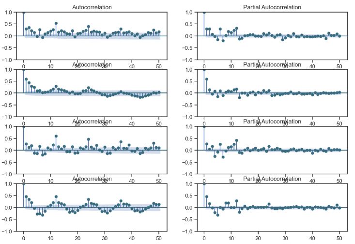
- Plotting ACF and PACF for 1st differences of 4 sales types: a, b, c, and d (from top to bottom)
# figure for subplots
plt.figure(figsize = (12, 8))

# acf and pacf for A
plt.subplot(421); plot_acf(first_diff_a, lags = 50, ax = plt.gca(), color = c)
plt.subplot(422); plot_pacf(first_diff_a, lags = 50, ax = plt.gca(), color = c)

# acf and pacf for B
plt.subplot(423); plot_acf(first_diff_b, lags = 50, ax = plt.gca(), color = c)
plt.subplot(424); plot_pacf(first_diff_b, lags = 50, ax = plt.gca(), color = c)

# acf and pacf for C
plt.subplot(425); plot_acf(first_diff_c, lags = 50, ax = plt.gca(), color = c)
plt.subplot(426); plot_pacf(first_diff_c, lags = 50, ax = plt.gca(), color = c)

# acf and pacf for D
plt.subplot(427); plot_acf(first_diff_d, lags = 50, ax = plt.gca(), color = c)
plt.subplot(428); plot_pacf(first_diff_d, lags = 50, ax = plt.gca(), color = c)

plt.show()
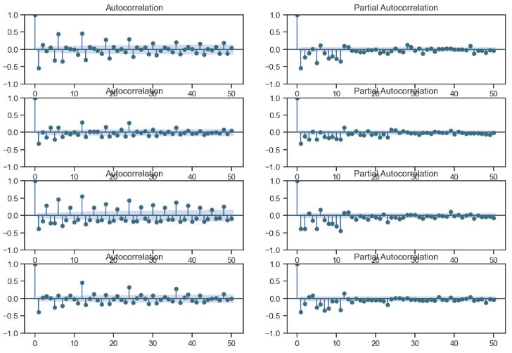
- Performing sales (a) SARIMA predictions
import warnings
warnings.filterwarnings("ignore")
#Data Manipulation and Treatment
import numpy as np
import pandas as pd
from datetime import datetime
#Plotting and Visualizations
import matplotlib.pyplot as plt
%matplotlib inline
import seaborn as sns
from scipy import stats
import itertools
#Scikit-Learn for Modeling
from sklearn import model_selection
from sklearn.ensemble import RandomForestRegressor
from sklearn import metrics
# statistics
#from statsmodels.tsa.arima_model import ARIMA
import statsmodels.api as sm
from statsmodels.distributions.empirical_distribution import ECDF
# time series analysis
from statsmodels.tsa.seasonal import seasonal_decompose
from statsmodels.graphics.tsaplots import plot_acf, plot_pacf
sarima_mod_a = sm.tsa.statespace.SARIMAX(sales_a, trend='n', order=(11,1,0), seasonal_order=(2,1,0,12)).fit()
print(sarima_mod_a.summary())
SARIMAX Results
===========================================================================================
Dep. Variable:                               Sales   No. Observations:                  780
Model:             SARIMAX(11, 1, 0)x(2, 1, 0, 12)   Log Likelihood               -6588.653
Date:                             Sun, 10 Dec 2023   AIC                          13205.306
Time:                                     19:04:36   BIC                          13270.300
Sample:                                          0   HQIC                         13230.323
                                             - 780
Covariance Type:                               opg
==============================================================================
                 coef    std err          z      P>|z|      [0.025      0.975]
------------------------------------------------------------------------------
ar.L1         -0.7897      0.030    -26.674      0.000      -0.848      -0.732
ar.L2         -0.4988      0.045    -11.078      0.000      -0.587      -0.411
ar.L3         -0.4437      0.046     -9.596      0.000      -0.534      -0.353
ar.L4         -0.3903      0.040     -9.683      0.000      -0.469      -0.311
ar.L5         -0.4298      0.045     -9.519      0.000      -0.518      -0.341
ar.L6         -0.2008      0.050     -4.032      0.000      -0.298      -0.103
ar.L7         -0.3278      0.050     -6.574      0.000      -0.425      -0.230
ar.L8         -0.3566      0.052     -6.873      0.000      -0.458      -0.255
ar.L9         -0.2854      0.052     -5.505      0.000      -0.387      -0.184
ar.L10        -0.2912      0.046     -6.344      0.000      -0.381      -0.201
ar.L11        -0.0715      0.044     -1.613      0.107      -0.158       0.015
ar.S.L12      -0.5634      0.045    -12.489      0.000      -0.652      -0.475
ar.S.L24      -0.2636      0.036     -7.288      0.000      -0.335      -0.193
sigma2      1.688e+06    6.1e+04     27.678      0.000    1.57e+06    1.81e+06
===================================================================================
Ljung-Box (L1) (Q):                   0.02   Jarque-Bera (JB):               408.73
Prob(Q):                              0.88   Prob(JB):                         0.00
Heteroskedasticity (H):               1.13   Skew:                            -0.25
Prob(H) (two-sided):                  0.32   Kurtosis:                         6.54
===================================================================================
- Plotting SARIMA model (a) residual distribution, ACF and PACF
residual_plot(sarima_mod_a)
NormaltestResult(statistic=74.64183175409748, pvalue=6.190591898477747e-17)
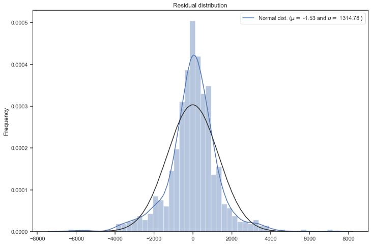

- Plotting actual sales (a) data (blue) vs SARIMA predictions (red)
plt.figure(figsize=(14,6))

plt.rcParams.update({'font.size': 16})
plt.plot(mydata_a, c='red')
plt.plot(sarima_mod_a_train.fittedvalues, c='blue')
plt.ylabel("Sales")
plt.xlabel("Time")
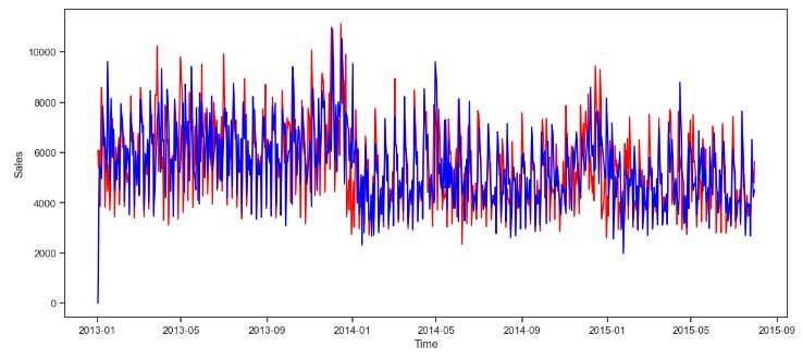
CO2 Concentration Data – 1. SARIMA Predictions
- Let’s discuss the monthly mean atmospheric carbon dioxide (CO2) concentration measured at Mauna Loa Observatory, Hawaii, and downloaded from ESRL at NOAA in October, 2016.
- This monthly data has a clear trend and seasonality across the sample, as shown here.
- Setting up the workspace
import sys
import pandas as pd
import numpy as np
import matplotlib.pylab as plt
%matplotlib inline
from matplotlib.pylab import rcParams
rcParams['figure.figsize'] = (12, 4)

import statsmodels.api as sm
from statsmodels.tsa.stattools import adfuller
from statsmodels.tsa.stattools import acf, pacf
from statsmodels.graphics.tsaplots import plot_acf, plot_pacf
from statsmodels.stats.stattools import durbin_watson as DW
from statsmodels.regression._prediction import get_prediction
from datetime import datetime
- Reading the input dataset
# Get the data
df = pd.read_csv('co2-ppm-mauna-loa-1958_03-2016_09.csv')
print(df.head())
print()
print(df.dtypes)
  Year  Month  Decimal Date  Average  Interpolated  Trend (Seasonal Corr)  \
0  1958      3      1958.208   315.71        315.71                 314.62
1  1958      4      1958.292   317.45        317.45                 315.29
2  1958      5      1958.375   317.50        317.50                 314.71
3  1958      6      1958.458   -99.99        317.10                 314.85
4  1958      7      1958.542   315.86        315.86                 314.98

   # Days
0      -1
1      -1
2      -1
3      -1
4      -1

Year                       int64
Month                      int64
Decimal Date             float64
Average                  float64
Interpolated             float64
Trend (Seasonal Corr)    float64
# Days                     int64
dtype: object
# The data is the monthly average CO2 (interpolated for missing months),
# so use the 15th day of the month (average day for most months)

# date_index = pd.to_datetime({'year':df['Year'], 'month':df['Month'], 'day':'15'})
# cols = ['interpolated_CO2']
data = pd.DataFrame(
    np.array(df['Interpolated']),
    index=pd.to_datetime({'year':df['Year'], 'month':df['Month'], 'day':'15'}),
    columns=['interpolated_CO2'])

print(data.head())
print()
print(data.tail())
print()
print(data.dtypes)
interpolated_CO2
1958-03-15            315.71
1958-04-15            317.45
1958-05-15            317.50
1958-06-15            317.10
1958-07-15            315.86

            interpolated_CO2
2016-05-15            407.70
2016-06-15            406.81
2016-07-15            404.39
2016-08-15            402.25
2016-09-15            401.03

interpolated_CO2    float64
dtype: object
- Selecting the training set and plotting the data
df_train = pd.DataFrame(data['interpolated_CO2']['2004':'2010'])

plt.plot(data, label='Whole series')
plt.plot(df_train, label='Training dataset')
plt.xlabel('Year')
plt.ylabel('CO2 concentration (ppm)')
plt.legend(loc='best');
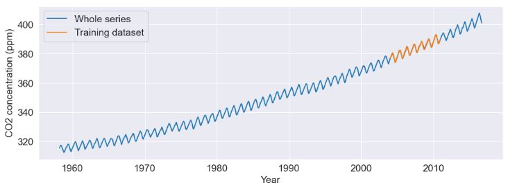
- Remove trend in mean by differencing and try seasonal differencing to remove the 12-month seasonal period
df_train['Differenced'] = df_train['interpolated_CO2'] - df_train['interpolated_CO2'].shift(1)
df_train['Diff_Seasonal'] = df_train['Differenced'] - df_train['Differenced'].shift(12)
- Check ACF and PACF of df_train[‘Diff_Seasonal’]
# Make autocorrelation plots

def test_acfs(time_series, num_lags):
    fig = plt.figure()
    ax1 = fig.add_subplot(211)
    fig = plot_acf(time_series, lags=num_lags, ax=ax1)
    ax2 = fig.add_subplot(212)
    fig = plot_pacf(time_series, lags=num_lags, ax=ax2)
    plt.tight_layout()
test_acfs(df_train['Diff_Seasonal'].dropna(), 30)
![ACF and PACF of df_train['Diff_Seasonal']](https://newdigitals.org/wp-content/uploads/2024/01/co2_diff_acf_pacf.jpg?w=745)
- Fitting the 1st model
def make_SARIMAX(time_series, terms1, terms2):
    # terms: (p,d,q) and (P,D,Q,s)
    # s is the peridicity (e.g., 12 for 12 months)
    model = sm.tsa.SARIMAX(
        time_series,
        order=(terms1[0],terms1[1],terms1[2]),
        seasonal_order=(terms2[0],terms2[1],terms2[2],terms2[3]))

    model_results = model.fit()
    model_fit = model_results.predict()

    # Visualize the model
    # Use model data starting after the first period to avoid the MA offset
    fig = plt.figure()
    plt.plot(time_series, label='Data')
    plt.plot(model_fit[13:], label='Model')
    plt.title('Model Fit')
    plt.legend(loc='best')
    plt.ylabel('CO2 concentration (ppm)')

    # Quantify the fit
    print(model_results.summary())

    return model, model_fit, model_results

# Make the first model
model1, model1_fit, model1_results = make_SARIMAX(df_train['interpolated_CO2'],[0,1,0],[1,1,1,12])

                                      SARIMAX Results
============================================================================================
Dep. Variable:                     interpolated_CO2   No. Observations:                   84
Model:             SARIMAX(0, 1, 0)x(1, 1, [1], 12)   Log Likelihood                 -34.056
Date:                              Sat, 23 Dec 2023   AIC                             74.111
Time:                                      13:31:56   BIC                             80.899
Sample:                                           0   HQIC                            76.811
                                               - 84
Covariance Type:                                opg
==============================================================================
                 coef    std err          z      P>|z|      [0.025      0.975]
------------------------------------------------------------------------------
ar.S.L12       0.2510      0.377      0.666      0.506      -0.488       0.990
ma.S.L12      -0.9957     23.323     -0.043      0.966     -46.708      44.717
sigma2         0.1188      2.739      0.043      0.965      -5.250       5.488
===================================================================================
Ljung-Box (L1) (Q):                   3.89   Jarque-Bera (JB):                 1.59
Prob(Q):                              0.05   Prob(JB):                         0.45
Heteroskedasticity (H):               0.91   Skew:                             0.35
Prob(H) (two-sided):                  0.83   Kurtosis:                         3.22
===================================================================================
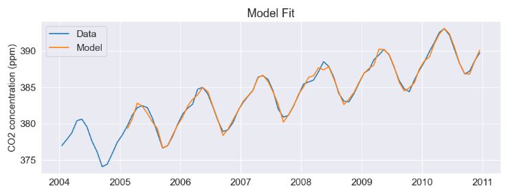
- Fitting the 2nd model
# Try another model that includes two MA terms.
model2, model2_fit, model2_results = make_SARIMAX(df_train['interpolated_CO2'],[0,1,2],[1,1,1,12])

    SARIMAX Results
============================================================================================
Dep. Variable:                     interpolated_CO2   No. Observations:                   84
Model:             SARIMAX(0, 1, 2)x(1, 1, [1], 12)   Log Likelihood                 -27.499
Date:                              Sat, 23 Dec 2023   AIC                             64.997
Time:                                      13:32:00   BIC                             76.311
Sample:                                           0   HQIC                            69.496
                                               - 84
Covariance Type:                                opg
==============================================================================
                 coef    std err          z      P>|z|      [0.025      0.975]
------------------------------------------------------------------------------
ma.L1         -0.4252      0.105     -4.050      0.000      -0.631      -0.219
ma.L2         -0.2679      0.161     -1.666      0.096      -0.583       0.047
ar.S.L12       0.2579      0.334      0.773      0.439      -0.396       0.912
ma.S.L12      -0.9957     19.278     -0.052      0.959     -38.781      36.789
sigma2         0.0981      1.872      0.052      0.958      -3.570       3.767
===================================================================================
Ljung-Box (L1) (Q):                   0.10   Jarque-Bera (JB):                 0.13
Prob(Q):                              0.76   Prob(JB):                         0.94
Heteroskedasticity (H):               1.03   Skew:                            -0.10
Prob(H) (two-sided):                  0.94   Kurtosis:                         3.01
===================================================================================
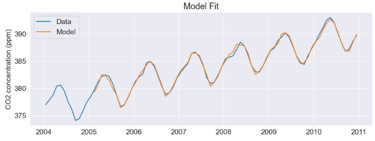
- Try an out-of-sample prediction using model 1.
# Make a prediction using model results
# ts should have indices that are older than the prediction range so
# that the two ranges overlap.
# pred_range is a list of two date strings bracketing the prediction

def make_pred(ts, model_res, pred_range):
    # Define data within range of prediction dates
    ts_pred_range = ts.loc[pred_range[0]:pred_range[1]]

    # Get the prediction
    # get_prediction requires ordinal index values
    pred_results = model_res.get_prediction(
        start=ts.index.get_loc(pred_range[0]),
        end=ts.index.get_loc(pred_range[1]))
    df_pred_summary = pred_results.summary_frame(alpha=0.05)

    # Add date indices to the prediction values
    df_pred_summary['date_time'] = ts_pred_range.index
    df_pred_summary.set_index('date_time', inplace=True)

    # Plot the prediction with the hold out data
    compare_prediction(ts_pred_range, df_pred_summary)

# Compare prediction with original series.  Includes
# a subplot of std err of mean,
# which is handy for seeing where the calibration data
# stops and the forecast begins.

def compare_prediction(ts_orig, df_pred):
    fig = plt.subplots(2, 1, sharex=True)
    plt.subplot(2,1,1)
    plt.plot(ts_orig, 'b', label='Data')
    plt.plot(df_pred['mean'], 'g', label='Prediction')
    plt.plot(df_pred['mean_ci_lower'], 'r:', label='95% CI')
    plt.plot(df_pred['mean_ci_upper'], 'r:', label='_nolegend_')
    plt.ylabel('CO2 concentration (ppm)')
    plt.legend(loc='best')

    plt.subplot(2,1,2)
    plt.plot(df_pred['mean_se'], label='Std Error of Mean')
    plt.xlabel('Year')
    plt.ylabel('Standard Error of Mean')
make_pred(
    pd.DataFrame(data['interpolated_CO2'][df_train.index[0]:]),
    model1_results,
    ['2010-12-15', '2016-09-15'])

- Creating a model 2 for use in out-of-sample predictions
# Make ordinal indices from forecast date strings

def make_forecast_ind(df, forecast_range):
    # Format the dates
    date1 = pd.to_datetime(forecast_range[0])
    date2 = pd.to_datetime(forecast_range[1])

    # Get the start date index
    # Ensure the start date is within the df index
    date1_ord = len(df) - 1
    if date1 < df.index[date1_ord]:
        date1_ord = df.index.get_loc(date1)


    # Calculate the end date index from the number of months in the range
    # Get the numbers of years and months
    date1_parsed = forecast_range[0].split('-')
    date2_parsed = forecast_range[1].split('-')
    num_years = int(date2_parsed[0]) - int(date1_parsed[0])
    num_months = int(date2_parsed[1]) - int(date1_parsed[1])

    # Check some conditions and calculate the number of months
    if num_months > 12:
        print('Months cannot exceed 12.  Try again.')
        print('Setting date range to 0.')
        range_in_months = 0
    else:
        if num_years > 0:
            num_years_as_months = num_years * 12
            range_in_months = num_years_as_months + num_months
        elif num_years < 0:
            print('End date must be after start date.')
            print('Setting date range to 0.')
            range_in_months = 0
        elif num_years == 0 and num_months < 0:
            print('End date must be after start date.')
            print('Setting date range to 0.')
            range_in_months = 0

    # Sum the months to find the last ordinal index of the range
    date2_ord = date1_ord + range_in_months

    return date1_ord, date2_ord, date1, date2
df_last = pd.DataFrame(data['interpolated_CO2']['2010':])
#df_last.tail()
# Choose forecast date range and create indices for modeling
forecast_date_range = ['2016-09-15', '2019-09-15']
begin_date_ord, end_date_ord, begin_date, end_date = make_forecast_ind(df_last, forecast_date_range)
# Create model for use in out-of-sample predictions
model2_forecast, model2_forecast_fit, model2_forecast_results = make_SARIMAX(
    df_last,[0,1,2],[1,1,1,12])
                                      SARIMAX Results
============================================================================================
Dep. Variable:                     interpolated_CO2   No. Observations:                   81
Model:             SARIMAX(0, 1, 2)x(1, 1, [1], 12)   Log Likelihood                 -34.551
Date:                              Sat, 23 Dec 2023   AIC                             79.102
Time:                                      13:32:20   BIC                             90.199
Sample:                                           0   HQIC                            83.499
                                               - 81
Covariance Type:                                opg
==============================================================================
                 coef    std err          z      P>|z|      [0.025      0.975]
------------------------------------------------------------------------------
ma.L1         -0.4012      0.151     -2.653      0.008      -0.698      -0.105
ma.L2         -0.0643      0.115     -0.559      0.576      -0.290       0.161
ar.S.L12      -0.3037      0.215     -1.415      0.157      -0.724       0.117
ma.S.L12      -0.3785      0.179     -2.113      0.035      -0.730      -0.027
sigma2         0.1484      0.031      4.745      0.000       0.087       0.210
===================================================================================
Ljung-Box (L1) (Q):                   0.09   Jarque-Bera (JB):                 0.77
Prob(Q):                              0.77   Prob(JB):                         0.68
Heteroskedasticity (H):               1.39   Skew:                             0.26
Prob(H) (two-sided):                  0.44   Kurtosis:                         3.06
===================================================================================
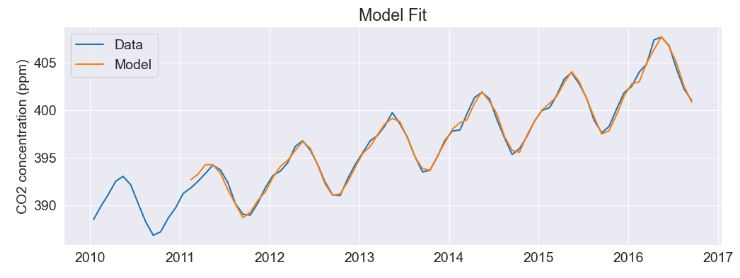
- Get the forecast model 2 and perform predictions
# Get the forecast model
forecast_results = model2_forecast_results.get_prediction(start=begin_date_ord, end=end_date_ord)
forecast_summary = forecast_results.summary_frame(alpha=0.05)
# Prediction

# Convert dates to dataframe indices for appending to data
future_dates = pd.date_range(start=forecast_date_range[0], end=forecast_date_range[1], freq='2SMS')
forecast_summary_dates = forecast_summary.set_index(future_dates)

# Plot the results to see the forecast
plt.plot(df_last, 'b', label='Data')
plt.plot(forecast_summary_dates['mean'][begin_date:end_date], 'g', label='Forecast')
plt.plot(forecast_summary_dates['mean_ci_lower'][begin_date:end_date], 'r:', label='95% CI')
plt.plot(forecast_summary_dates['mean_ci_upper'][begin_date:end_date], 'r:', label='_nolegend_')
plt.ylabel('CO2 concentration (ppm)')
plt.xlabel('Year')
plt.legend(loc='best')
#plt.savefig('CO2_forecast.png')

CO2 Concentration Data – 2. ARIMA Dynamic Forecast
- Here, we proceed to apply ARIMA – one of the most commonly used method for CO2 time-series forecasting.
- Input data preparation
import warnings
import itertools
import pandas as pd
import numpy as np
import statsmodels.api as sm
import matplotlib.pyplot as plt
plt.style.use('fivethirtyeight')
data = sm.datasets.co2.load_pandas()
y = data.data
# The 'MS' string groups the data in buckets by start of the month
y = y['co2'].resample('MS').mean()

# The term bfill means that we use the value before filling in missing values
y = y.fillna(y.bfill())

#print(y)
y.plot(figsize=(15, 6))
plt.show()

#CO2 levels vs Date
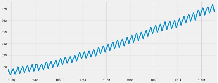
- Tuning the ARIMA parameters p, d and q
# Define the p, d and q parameters to take any value between 0 and 2
p = d = q = range(0, 2)

# Generate all different combinations of p, q and q triplets
pdq = list(itertools.product(p, d, q))

# Generate all different combinations of seasonal p, q and q triplets
seasonal_pdq = [(x[0], x[1], x[2], 12) for x in list(itertools.product(p, d, q))]

print('Examples of parameter combinations for Seasonal ARIMA...')
print('SARIMAX: {} x {}'.format(pdq[1], seasonal_pdq[1]))
print('SARIMAX: {} x {}'.format(pdq[1], seasonal_pdq[2]))
print('SARIMAX: {} x {}'.format(pdq[2], seasonal_pdq[3]))
print('SARIMAX: {} x {}'.format(pdq[2], seasonal_pdq[4]))
Examples of parameter combinations for Seasonal ARIMA...
SARIMAX: (0, 0, 1) x (0, 0, 1, 12)
SARIMAX: (0, 0, 1) x (0, 1, 0, 12)
SARIMAX: (0, 1, 0) x (0, 1, 1, 12)
SARIMAX: (0, 1, 0) x (1, 0, 0, 12)
warnings.filterwarnings("ignore") # specify to ignore warning messages

for param in pdq:
    for param_seasonal in seasonal_pdq:
        try:
            mod = sm.tsa.statespace.SARIMAX(y,
                                            order=param,
                                            seasonal_order=param_seasonal,
                                            enforce_stationarity=False,
                                            enforce_invertibility=False)

            results = mod.fit()

            print('ARIMA{}x{}12 - AIC:{}'.format(param, param_seasonal, results.aic))
        except:
            continue
ARIMA(0, 0, 0)x(0, 0, 0, 12)12 - AIC:7612.583429881011
ARIMA(0, 0, 0)x(0, 0, 1, 12)12 - AIC:6787.343624044046
ARIMA(0, 0, 0)x(0, 1, 0, 12)12 - AIC:1854.8282341411793
ARIMA(0, 0, 0)x(0, 1, 1, 12)12 - AIC:1596.7111727643992
ARIMA(0, 0, 0)x(1, 0, 0, 12)12 - AIC:1058.9388921320058
ARIMA(0, 0, 0)x(1, 0, 1, 12)12 - AIC:1056.2878474543522
ARIMA(0, 0, 0)x(1, 1, 0, 12)12 - AIC:1361.6578977897923
ARIMA(0, 0, 0)x(1, 1, 1, 12)12 - AIC:1044.7647913082933
ARIMA(0, 0, 1)x(0, 0, 0, 12)12 - AIC:6881.048754485544
ARIMA(0, 0, 1)x(0, 0, 1, 12)12 - AIC:6072.662327351689
ARIMA(0, 0, 1)x(0, 1, 0, 12)12 - AIC:1379.1941066953214
ARIMA(0, 0, 1)x(0, 1, 1, 12)12 - AIC:1241.4174716858438
ARIMA(0, 0, 1)x(1, 0, 0, 12)12 - AIC:1084.5829338880562
ARIMA(0, 0, 1)x(1, 0, 1, 12)12 - AIC:933.8572919274021
ARIMA(0, 0, 1)x(1, 1, 0, 12)12 - AIC:1119.5957893631296
ARIMA(0, 0, 1)x(1, 1, 1, 12)12 - AIC:807.091298750021
ARIMA(0, 1, 0)x(0, 0, 0, 12)12 - AIC:1675.808692302429
ARIMA(0, 1, 0)x(0, 0, 1, 12)12 - AIC:1240.2211199194044
ARIMA(0, 1, 0)x(0, 1, 0, 12)12 - AIC:633.4425587879977
ARIMA(0, 1, 0)x(0, 1, 1, 12)12 - AIC:337.7938547933855
ARIMA(0, 1, 0)x(1, 0, 0, 12)12 - AIC:619.9501758052422
ARIMA(0, 1, 0)x(1, 0, 1, 12)12 - AIC:376.9283760094577
ARIMA(0, 1, 0)x(1, 1, 0, 12)12 - AIC:478.3296908096461
ARIMA(0, 1, 0)x(1, 1, 1, 12)12 - AIC:323.0776499827083
ARIMA(0, 1, 1)x(0, 0, 0, 12)12 - AIC:1371.187260233787
ARIMA(0, 1, 1)x(0, 0, 1, 12)12 - AIC:1101.8410734302472
ARIMA(0, 1, 1)x(0, 1, 0, 12)12 - AIC:587.94797103039
ARIMA(0, 1, 1)x(0, 1, 1, 12)12 - AIC:302.49489996321256
ARIMA(0, 1, 1)x(1, 0, 0, 12)12 - AIC:584.4333533496758
ARIMA(0, 1, 1)x(1, 0, 1, 12)12 - AIC:337.1999051016703
ARIMA(0, 1, 1)x(1, 1, 0, 12)12 - AIC:433.08636080989186
ARIMA(0, 1, 1)x(1, 1, 1, 12)12 - AIC:281.5189758069086
ARIMA(1, 0, 0)x(0, 0, 0, 12)12 - AIC:1676.8881767362063
ARIMA(1, 0, 0)x(0, 0, 1, 12)12 - AIC:1241.9354689272566
ARIMA(1, 0, 0)x(0, 1, 0, 12)12 - AIC:624.2602350580995
ARIMA(1, 0, 0)x(0, 1, 1, 12)12 - AIC:341.2896617005996
ARIMA(1, 0, 0)x(1, 0, 0, 12)12 - AIC:579.3896923181578
ARIMA(1, 0, 0)x(1, 0, 1, 12)12 - AIC:370.59205674829855
ARIMA(1, 0, 0)x(1, 1, 0, 12)12 - AIC:476.0500428835895
ARIMA(1, 0, 0)x(1, 1, 1, 12)12 - AIC:327.5808594238757
ARIMA(1, 0, 1)x(0, 0, 0, 12)12 - AIC:1372.6085881650192
ARIMA(1, 0, 1)x(0, 0, 1, 12)12 - AIC:1199.488810591478
ARIMA(1, 0, 1)x(0, 1, 0, 12)12 - AIC:586.4485732478089
ARIMA(1, 0, 1)x(0, 1, 1, 12)12 - AIC:305.62738225336267
ARIMA(1, 0, 1)x(1, 0, 0, 12)12 - AIC:586.3305595671048
ARIMA(1, 0, 1)x(1, 0, 1, 12)12 - AIC:399.03053061183766
ARIMA(1, 0, 1)x(1, 1, 0, 12)12 - AIC:433.54694644704455
ARIMA(1, 0, 1)x(1, 1, 1, 12)12 - AIC:284.35964260553385
ARIMA(1, 1, 0)x(0, 0, 0, 12)12 - AIC:1324.3111127324546
ARIMA(1, 1, 0)x(0, 0, 1, 12)12 - AIC:1060.9351914446981
ARIMA(1, 1, 0)x(0, 1, 0, 12)12 - AIC:600.7412683004577
ARIMA(1, 1, 0)x(0, 1, 1, 12)12 - AIC:312.1329633757754
ARIMA(1, 1, 0)x(1, 0, 0, 12)12 - AIC:593.6637754936671
ARIMA(1, 1, 0)x(1, 0, 1, 12)12 - AIC:349.2091450970028
ARIMA(1, 1, 0)x(1, 1, 0, 12)12 - AIC:440.1375884441029
ARIMA(1, 1, 0)x(1, 1, 1, 12)12 - AIC:293.74262233316983
ARIMA(1, 1, 1)x(0, 0, 0, 12)12 - AIC:1262.654554246471
ARIMA(1, 1, 1)x(0, 0, 1, 12)12 - AIC:1052.0636724057626
ARIMA(1, 1, 1)x(0, 1, 0, 12)12 - AIC:581.309993514378
ARIMA(1, 1, 1)x(0, 1, 1, 12)12 - AIC:295.9374059170541
ARIMA(1, 1, 1)x(1, 0, 0, 12)12 - AIC:576.8647111604348
ARIMA(1, 1, 1)x(1, 0, 1, 12)12 - AIC:327.90491313011745
ARIMA(1, 1, 1)x(1, 1, 0, 12)12 - AIC:444.1243686516594
ARIMA(1, 1, 1)x(1, 1, 1, 12)12 - AIC:277.78040980734056
- Fitting the optimized model and plotting the key diagnostics
mod = sm.tsa.statespace.SARIMAX(y,
                                order=(1, 1, 1),
                                seasonal_order=(1, 1, 1, 12),
                                enforce_stationarity=False,
                                enforce_invertibility=False)

results = mod.fit()

print(results.summary().tables[1])
==============================================================================
                 coef    std err          z      P>|z|      [0.025      0.975]
------------------------------------------------------------------------------
ar.L1          0.3181      0.092      3.444      0.001       0.137       0.499
ma.L1         -0.6256      0.077     -8.177      0.000      -0.776      -0.476
ar.S.L12       0.0010      0.001      1.732      0.083      -0.000       0.002
ma.S.L12      -0.8766      0.026    -33.760      0.000      -0.928      -0.826
sigma2         0.0971      0.004     22.636      0.000       0.089       0.106
==============================================================================
results.plot_diagnostics(figsize=(15, 12))
plt.show()
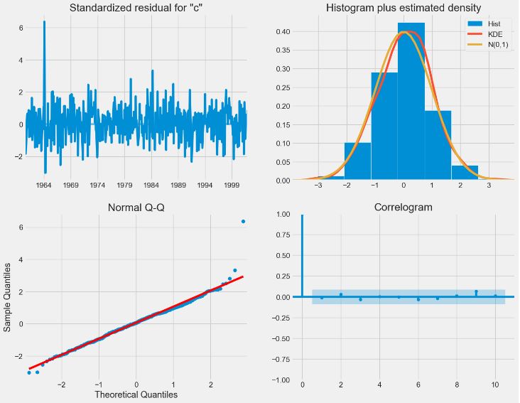
- Performing ARIMA predictions starting 1998-01-01
pred = results.get_prediction(start=pd.to_datetime('1998-01-01'), dynamic=False)
pred_ci = pred.conf_int()
fig, ax = plt.subplots(figsize=(10, 6))
ax = y['1990':].plot(label='observed')
pred.predicted_mean.plot(ax=ax, label='One-step ahead Forecast', alpha=.7)

ax.fill_between(pred_ci.index,
                pred_ci.iloc[:, 0],
                pred_ci.iloc[:, 1], color='k', alpha=.2)

ax.set_xlabel('Date')
ax.set_ylabel('CO2 Levels')
plt.legend()

plt.show()
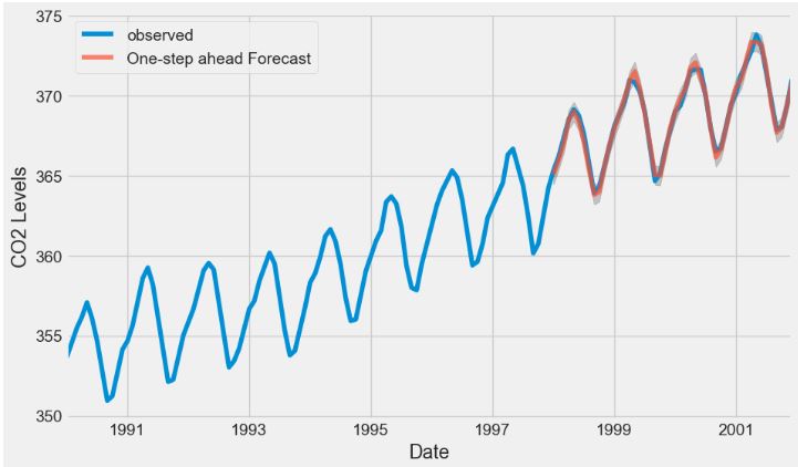
- Computing MSA of the predicted CO2 values
y_forecasted = pred.predicted_mean
y_truth = y['1998-01-01':]

# Compute the mean square error
mse = ((y_forecasted - y_truth) ** 2).mean()
print('The Mean Squared Error of our forecasts is {}'.format(round(mse, 2)))

The Mean Squared Error of our forecasts is 0.07
- Performing the dynamic ARIMA forecast
pred_dynamic = results.get_prediction(start=pd.to_datetime('1998-01-01'), dynamic=True, full_results=True)
pred_dynamic_ci = pred_dynamic.conf_int()
ax = y['1990':].plot(label='observed', figsize=(10, 6))
pred_dynamic.predicted_mean.plot(label='Dynamic Forecast', ax=ax)

ax.fill_between(pred_dynamic_ci.index,
                pred_dynamic_ci.iloc[:, 0],
                pred_dynamic_ci.iloc[:, 1], color='k', alpha=.25)

ax.fill_betweenx(ax.get_ylim(), pd.to_datetime('1998-01-01'), y.index[-1],
                 alpha=.1, zorder=-1)

ax.set_xlabel('Date')
ax.set_ylabel('CO2 Levels')

plt.legend(loc='upper left')
plt.show()
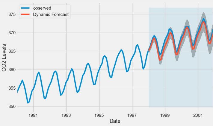
- Performing the long-term ARIMA dynamic forecast starting 1998-01-01 with steps=500
# Extract the predicted and true values of our time series
y_forecasted = pred_dynamic.predicted_mean
y_truth = y['1998-01-01':]

# Compute the mean square error
mse = ((y_forecasted - y_truth) ** 2).mean()
print('The Mean Squared Error of our forecasts is {}'.format(round(mse, 2)))

The Mean Squared Error of our forecasts is 1.01

# Get forecast 500 steps ahead in future
pred_uc = results.get_forecast(steps=500)

# Get confidence intervals of forecasts
pred_ci = pred_uc.conf_int()

ax = y.plot(label='observed', figsize=(10, 6))
pred_uc.predicted_mean.plot(ax=ax, label='Forecast')
ax.fill_between(pred_ci.index,
                pred_ci.iloc[:, 0],
                pred_ci.iloc[:, 1], color='k', alpha=.25)
ax.set_xlabel('Date')
ax.set_ylabel('CO2 Levels')

plt.legend(loc='upper left')
plt.show()
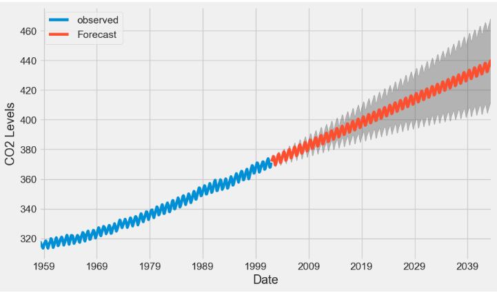
CO2 Concentration Data – 3. ML Regression
- We have examined the so-called traditional models for TSF, such as the SARIMAX family of models and exponential smoothing.
- In this section, we will formulate a TSF problem as a supervised ML regression, allowing us to use a great variety of SciKit-Learn estimators (decision trees, random forests, gradient boosting, etc.).
- Reading the input CO2 data
import numpy as np
import pandas as pd
import statsmodels.api as sm
import matplotlib.pyplot as plt
data = sm.datasets.co2.load_pandas().data
fig, ax = plt.subplots(figsize=(16, 11))
ax.plot(data['co2'])
ax.set_xlabel('Time')
ax.set_ylabel('CO2 concentration (ppmw)')
fig.autofmt_xdate()
plt.tight_layout()

- Data preparation
data = data.interpolate()
df = data.copy()
df['y'] = df['co2'].shift(-1)
#df.head(5)
df = data.copy()
df['y'] = df['co2'].shift(-1)
#df
train = df[:-104]
test = df[-104:]
test = test.drop(test.tail(1).index) # Drop last row
test = test.copy()
test['baseline_pred'] = test['co2']
test.head(10)
	          co2	y	baseline_pred
2000-01-08	368.5	369.0	368.5
2000-01-15	369.0	369.8	369.0
2000-01-22	369.8	369.2	369.8
2000-01-29	369.2	369.1	369.2
2000-02-05	369.1	369.6	369.1
2000-02-12	369.6	369.3	369.6
2000-02-19	369.3	369.5	369.3
2000-02-26	369.5	370.0	369.5
2000-03-04	370.0	370.0	370.0
2000-03-11	370.0	370.9	370.0
- Training the Decision Tree Regressor
from sklearn.tree import DecisionTreeRegressor

X_train = train['co2'].values.reshape(-1,1)
y_train = train['y'].values.reshape(-1,1)
X_test = test['co2'].values.reshape(-1,1)

# Initialize the model
dt_reg = DecisionTreeRegressor(random_state=42)

# Fit the model
dt_reg.fit(X=X_train, y=y_train)

# Make predictions
dt_pred = dt_reg.predict(X_test)

# Assign predictions to a new column in test
test['dt_pred'] = dt_pred

# view the model
#test.head(10)
- Training the Gradient Boosting Regressor
from sklearn.ensemble import GradientBoostingRegressor
gbr = GradientBoostingRegressor(random_state=42)
gbr.fit(X_train, y=y_train.ravel())
gbr_pred = gbr.predict(X_test)
test['gbr_pred'] = gbr_pred

#Check the output
#test.head(10)
- Computing MAPE for 3 trained models
def mape(y_true, y_pred):
    return round(np.mean(np.abs((y_true - y_pred) / y_true)) * 100, 2)

baseline_mape = mape(test['y'], test['baseline_pred'])
dt_mape = mape(test['y'], test['dt_pred'])
gbr_mape = mape(test['co2'], test['gbr_pred'])
# Generate bar plot
fig, ax = plt.subplots(figsize=(7, 5))
x = ['Baseline', 'Decision Tree', 'Gradient Boosting']
y = [baseline_mape, dt_mape, gbr_mape]
ax.bar(x, y, width=0.4)
ax.set_xlabel('Regressor models')
ax.set_ylabel('MAPE (%)')
ax.set_ylim(0, 0.3)
for index, value in enumerate(y):
    plt.text(x=index, y=value + 0.02, s=str(value), ha='center')

plt.tight_layout()

- Implementing the multi-output windowed ML regression as Regressor Chain that predicts a sequence of future time steps using a sequence of past observations.
def window_input(window_length: int, data: pd.DataFrame) -> pd.DataFrame:

    df = data.copy()

    i = 1
    while i < window_length:
        df[f'x_{i}'] = df['co2'].shift(-i)
        i = i + 1

    if i == window_length:
        df['y'] = df['co2'].shift(-i)

    # Drop rows where there is a NaN
    df = df.dropna(axis=0)

    return df
new_df = window_input(5, data)
#new_df
- Train/test windowed data splitting with test_size=0.3
from sklearn.model_selection import train_test_split

X = new_df[['co2', 'x_1', 'x_2', 'x_3', 'x_4']].values
y = new_df['y'].values

X_train, X_test, y_train, y_test = train_test_split(X, y, test_size=0.3, random_state=42, shuffle=False)

baseline_pred = []

for row in X_test:
    baseline_pred.append(np.mean(row))
dt_reg_5 = DecisionTreeRegressor(random_state=42)

dt_reg_5.fit(X_train, y_train)

dt_reg_5_pred = dt_reg_5.predict(X_test)
def window_input_output(input_length: int, output_length: int, data: pd.DataFrame) -> pd.DataFrame:

    df = data.copy()

    i = 1
    while i < input_length:
        df[f'x_{i}'] = df['co2'].shift(-i)
        i = i + 1

    j = 0
    while j < output_length:
        df[f'y_{j}'] = df['co2'].shift(-output_length-j)
        j = j + 1

    df = df.dropna(axis=0)

    return df
seq_df = window_input_output(26, 26, data)
#seq_df

X_cols = [col for col in seq_df.columns if col.startswith('x')]

X_cols.insert(0, 'co2')

y_cols = [col for col in seq_df.columns if col.startswith('y')]
X_train = seq_df[X_cols][:-2].values
y_train = seq_df[y_cols][:-2].values

X_test = seq_df[X_cols][-2:].values
y_test = seq_df[y_cols][-2:].values
dt_seq = DecisionTreeRegressor(random_state=42)

dt_seq.fit(X_train, y_train)

dt_seq_preds = dt_seq.predict(X_test)
from sklearn.multioutput import RegressorChain

gbr_seq = GradientBoostingRegressor(random_state=42)

chained_gbr = RegressorChain(gbr_seq)

chained_gbr.fit(X_train, y_train)

gbr_seq_preds = chained_gbr.predict(X_test)
mape_dt_seq = mape(dt_seq_preds.reshape(1, -1), y_test.reshape(1, -1))
mape_gbr_seq = mape(gbr_seq_preds.reshape(1, -1), y_test.reshape(1, -1))
mape_baseline = mape(X_test.reshape(1, -1), y_test.reshape(1, -1))
# Generate the bar plot
fig, ax = plt.subplots()

x = ['Baseline', 'Decision Tree', 'Gradient Boosting']
y = [mape_baseline, mape_dt_seq, mape_gbr_seq]

ax.bar(x, y, width=0.4)
ax.set_xlabel('Regressor models')
ax.set_ylabel('MAPE (%)')
ax.set_ylim(0, 1)

for index, value in enumerate(y):
    plt.text(x=index, y=value + 0.05, s=str(value), ha='center')

plt.tight_layout()

- From the figure above, we can see that we have managed to train ML models that outperform the baseline model! Here, the Decision Tree model is the best performer in terms of MAPE.
fig, ax = plt.subplots(figsize=(10, 6))
ax.plot(np.arange(0, 26, 1), X_test[1], 'b-', label='input')
ax.plot(np.arange(26, 52, 1), y_test[1], marker='.', color='blue', label='Actual')
ax.plot(np.arange(26, 52, 1), X_test[1], marker='o', color='red', label='Baseline')
ax.plot(np.arange(26, 52, 1), dt_seq_preds[1], marker='^', color='green', label='Decision Tree')
ax.plot(np.arange(26, 52, 1), gbr_seq_preds[1], marker='P', color='black', label='Gradient Boosting')
ax.set_xlabel('Timesteps')
ax.set_ylabel('CO2 concentration (ppmv)')
plt.xticks(np.arange(1, 104, 52), np.arange(2000, 2002, 1))
plt.legend(loc='lower left')
fig.autofmt_xdate()
plt.tight_layout()
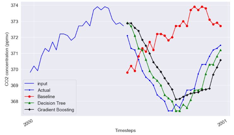
- Clearly, the Baseline prediction is way off, while the Decision Tree and Gradient Boosting TSF follow the actual values more closely.
- Now we have implemented and tested the framework to apply any ML regression for TSF along with the statistical models mentioned above.
- Read more here.
Unemployment/Interest Rate OLS
- In this section, we’ll walk through a linear regression using statsmodels.
- The input dataset consists of 2 independent variables representing the interest and unemployment rates.
- Preparing the input data and independent variables x, y
import pandas as pd
import statsmodels.api as sm

data = {'year': [2017,2017,2017,2017,2017,2017,2017,2017,2017,2017,2017,2017,2016,2016,2016,2016,2016,2016,2016,2016,2016,2016,2016,2016],
        'month': [12,11,10,9,8,7,6,5,4,3,2,1,12,11,10,9,8,7,6,5,4,3,2,1],
        'interest_rate': [2.75,2.5,2.5,2.5,2.5,2.5,2.5,2.25,2.25,2.25,2,2,2,1.75,1.75,1.75,1.75,1.75,1.75,1.75,1.75,1.75,1.75,1.75],
        'unemployment_rate': [5.3,5.3,5.3,5.3,5.4,5.6,5.5,5.5,5.5,5.6,5.7,5.9,6,5.9,5.8,6.1,6.2,6.1,6.1,6.1,5.9,6.2,6.2,6.1],
        'index_price': [1464,1394,1357,1293,1256,1254,1234,1195,1159,1167,1130,1075,1047,965,943,958,971,949,884,866,876,822,704,719]
        }

df = pd.DataFrame(data)

x = df[['interest_rate','unemployment_rate']]
y = df['index_price']

x = sm.add_constant(x)
- Fitting and printing the OLS model
model = sm.OLS(y, x).fit()
predictions = model.predict(x)

print_model = model.summary()
print(print_model)
 OLS Regression Results
==============================================================================
Dep. Variable:            index_price   R-squared:                       0.898
Model:                            OLS   Adj. R-squared:                  0.888
Method:                 Least Squares   F-statistic:                     92.07
Date:                Sat, 23 Dec 2023   Prob (F-statistic):           4.04e-11
Time:                        13:30:53   Log-Likelihood:                -134.61
No. Observations:                  24   AIC:                             275.2
Df Residuals:                      21   BIC:                             278.8
Df Model:                           2
Covariance Type:            nonrobust
=====================================================================================
                        coef    std err          t      P>|t|      [0.025      0.975]
-------------------------------------------------------------------------------------
const              1798.4040    899.248      2.000      0.059     -71.685    3668.493
interest_rate       345.5401    111.367      3.103      0.005     113.940     577.140
unemployment_rate  -250.1466    117.950     -2.121      0.046    -495.437      -4.856
==============================================================================
Omnibus:                        2.691   Durbin-Watson:                   0.530
Prob(Omnibus):                  0.260   Jarque-Bera (JB):                1.551
Skew:                          -0.612   Prob(JB):                        0.461
Kurtosis:                       3.226   Cond. No.                         394.
==============================================================================
- Fitting the SciKit-Learn Linear Regression model
import pandas as pd
from sklearn import linear_model
import statsmodels.api as sm
# with sklearn
regr = linear_model.LinearRegression()
regr.fit(x, y)

print('Intercept: \n', regr.intercept_)
print('Coefficients: \n', regr.coef_)
Intercept:
 1798.403977625855
Coefficients:
 [ 345.54008701 -250.14657137]
- We can see that the intercept and 2 coefficients are the same for both linear models.
- Adjusted. R-squared reflects the fit of the model. R-squared value of 0.888 indicates a good fit.
- P >|t| is the p-value. A p-value of less than 0.05 is considered to be statistically significant.
Oil Production in Saudi Arabia
- Let’s look at the annual oil production in Saudi Arabia
import os
import numpy as np
import pandas as pd
import matplotlib.pyplot as plt
from statsmodels.tsa.api import ExponentialSmoothing, SimpleExpSmoothing, Holt

%matplotlib inline

data = [
    446.6565,
    454.4733,
    455.663,
    423.6322,
    456.2713,
    440.5881,
    425.3325,
    485.1494,
    506.0482,
    526.792,
    514.2689,
    494.211,
]
index = pd.date_range(start="1996", end="2008", freq="A")
oildata = pd.Series(data, index)
- Let’s use the Simple Exponential Smoothing method to forecast the oil production data oildata
fig, ax = plt.subplots(figsize=(10, 6))
ax = oildata.plot()
ax.set_xlabel("Year")
ax.set_ylabel("Oil (millions of tonnes)")
print("Oil production in Saudi Arabia from 1996 to 2007.")
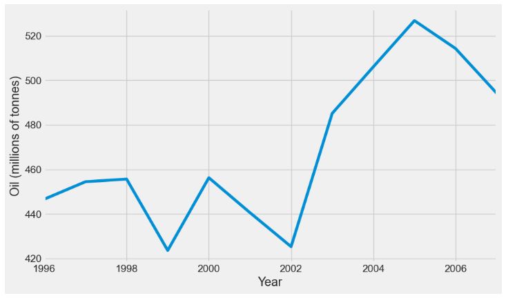
- Here we run three variants of simple exponential smoothing:
- In
fit1we do not use the auto optimization but instead choose to explicitly provide the model with the alpha=0.2 parameter - In
fit2as above we choose an alpha=0.6 - In
fit3we allow statsmodels to automatically find an optimized alpha value for us.
fit1 = SimpleExpSmoothing(oildata, initialization_method="heuristic").fit(
    smoothing_level=0.2, optimized=False
)
fcast1 = fit1.forecast(3).rename(r"$\alpha=0.2$")
fit2 = SimpleExpSmoothing(oildata, initialization_method="heuristic").fit(
    smoothing_level=0.6, optimized=False
)
fcast2 = fit2.forecast(3).rename(r"$\alpha=0.6$")
fit3 = SimpleExpSmoothing(oildata, initialization_method="estimated").fit()
fcast3 = fit3.forecast(3).rename(r"$\alpha=%s$" % fit3.model.params["smoothing_level"])

plt.figure(figsize=(12, 8))
plt.plot(oildata, marker="o", color="black")
plt.plot(fit1.fittedvalues, marker="o", color="blue")
(line1,) = plt.plot(fcast1, marker="o", color="blue")
plt.plot(fit2.fittedvalues, marker="o", color="red")
(line2,) = plt.plot(fcast2, marker="o", color="red")
plt.plot(fit3.fittedvalues, marker="o", color="green")
(line3,) = plt.plot(fcast3, marker="o", color="green")
plt.legend([line1, line2, line3], [fcast1.name, fcast2.name, fcast3.name])
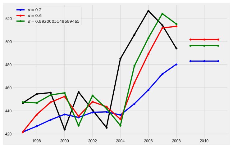
- Here, the black curve designates actual time series data.
Air Pollution & the Holt’s Method
- Lets take a look at another example. This time we use the air pollution data and the Holt’s Method. We will fit three examples again.
- In
fit1we again choose not to use the optimizer and provide explicit values for alpha=0.2 and beta=0.8. - In
fit2we do the same as infit1but choose to use an exponential model rather than a Holt’s additive model. - In
fit3we used a damped versions of the Holt’s additive model but allow the dampening parameter phi to be optimized while fixing the values for alpha=0.2 and beta=0.8. - Reading the input data
data = [
    17.5534,
    21.86,
    23.8866,
    26.9293,
    26.8885,
    28.8314,
    30.0751,
    30.9535,
    30.1857,
    31.5797,
    32.5776,
    33.4774,
    39.0216,
    41.3864,
    41.5966,
]
index = pd.date_range(start="1990", end="2005", freq="A")
air = pd.Series(data, index)
- Implementing the Holt’s method
fit1 = Holt(air, initialization_method="estimated").fit(
    smoothing_level=0.8, smoothing_trend=0.2, optimized=False
)
fcast1 = fit1.forecast(5).rename("Holt's linear trend")
fit2 = Holt(air, exponential=True, initialization_method="estimated").fit(
    smoothing_level=0.8, smoothing_trend=0.2, optimized=False
)
fcast2 = fit2.forecast(5).rename("Exponential trend")
fit3 = Holt(air, damped_trend=True, initialization_method="estimated").fit(
    smoothing_level=0.8, smoothing_trend=0.2
)
fcast3 = fit3.forecast(5).rename("Additive damped trend")

plt.figure(figsize=(12, 8))
plt.plot(air, marker="o", color="black")
plt.plot(fit1.fittedvalues, color="blue")
(line1,) = plt.plot(fcast1, marker="o", color="blue")
plt.plot(fit2.fittedvalues, color="red")
(line2,) = plt.plot(fcast2, marker="o", color="red")
plt.plot(fit3.fittedvalues, color="green")
(line3,) = plt.plot(fcast3, marker="o", color="green")
plt.legend([line1, line2, line3], [fcast1.name, fcast2.name, fcast3.name])

- Here, the black curve designates actual time series data.
Livestock, Sheep in Asia
- Let’s look at some seasonally adjusted livestock data
data = [
    263.9177,
    268.3072,
    260.6626,
    266.6394,
    277.5158,
    283.834,
    290.309,
    292.4742,
    300.8307,
    309.2867,
    318.3311,
    329.3724,
    338.884,
    339.2441,
    328.6006,
    314.2554,
    314.4597,
    321.4138,
    329.7893,
    346.3852,
    352.2979,
    348.3705,
    417.5629,
    417.1236,
    417.7495,
    412.2339,
    411.9468,
    394.6971,
    401.4993,
    408.2705,
    414.2428,
]
index = pd.date_range(start="1970", end="2001", freq="A")
livestock2 = pd.Series(data, index)
- Let’s fit the following 5 Holt’s models
fit1 = SimpleExpSmoothing(livestock2, initialization_method="estimated").fit()
fcast1 = fit1.forecast(9).rename("SES")
fit2 = Holt(livestock2, initialization_method="estimated").fit()
fcast2 = fit2.forecast(9).rename("Holt's")
fit3 = Holt(livestock2, exponential=True, initialization_method="estimated").fit()
fcast3 = fit3.forecast(9).rename("Exponential")
fit4 = Holt(livestock2, damped_trend=True, initialization_method="estimated").fit(
    damping_trend=0.98
)
fcast4 = fit4.forecast(9).rename("Additive Damped")
fit5 = Holt(
    livestock2, exponential=True, damped_trend=True, initialization_method="estimated"
).fit()
fcast5 = fit5.forecast(9).rename("Multiplicative Damped")

ax = livestock2.plot(color="black", marker="o", figsize=(12, 8))
livestock3.plot(ax=ax, color="black", marker="o", legend=False)
fcast1.plot(ax=ax, color="red", legend=True)
fcast2.plot(ax=ax, color="green", legend=True)
fcast3.plot(ax=ax, color="blue", legend=True)
fcast4.plot(ax=ax, color="cyan", legend=True)
fcast5.plot(ax=ax, color="magenta", legend=True)
ax.set_ylabel("Livestock, sheep in Asia (millions)")
plt.show()
print(
    "Forecasting livestock, sheep in Asia: comparing forecasting performance of non-seasonal methods."
)
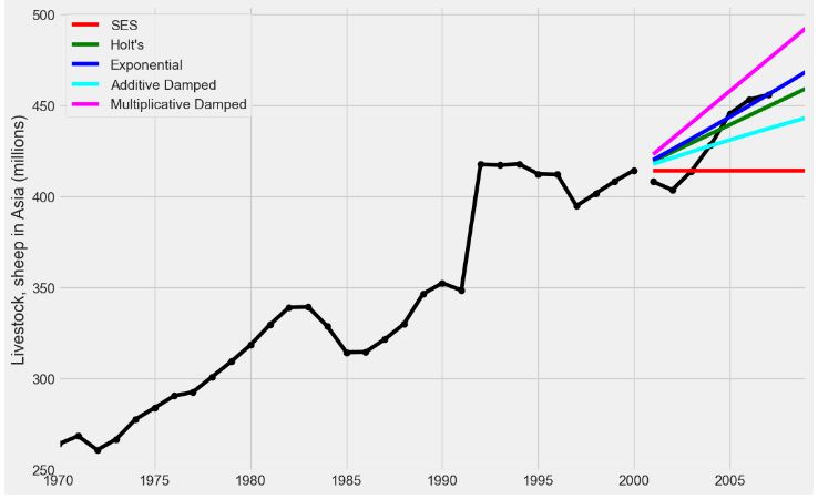
Forecasting livestock, sheep in Asia: comparing forecasting performance of non-seasonal methods.
International Visitor Nights in Australia
- Let’s look at forecasting international visitor nights in Australia using Holt-Winters method with both additive and multiplicative seasonality.
- Reading the input dataset
data = [
    41.7275,
    24.0418,
    32.3281,
    37.3287,
    46.2132,
    29.3463,
    36.4829,
    42.9777,
    48.9015,
    31.1802,
    37.7179,
    40.4202,
    51.2069,
    31.8872,
    40.9783,
    43.7725,
    55.5586,
    33.8509,
    42.0764,
    45.6423,
    59.7668,
    35.1919,
    44.3197,
    47.9137,
]
index = pd.date_range(start="2005", end="2010-Q4", freq="QS-OCT")
aust = pd.Series(data, index)
- Applying the following models to the above dataset
fit1 = ExponentialSmoothing(
    aust,
    seasonal_periods=4,
    trend="add",
    seasonal="add",
    use_boxcox=True,
    initialization_method="estimated",
).fit()
fit2 = ExponentialSmoothing(
    aust,
    seasonal_periods=4,
    trend="add",
    seasonal="mul",
    use_boxcox=True,
    initialization_method="estimated",
).fit()
fit3 = ExponentialSmoothing(
    aust,
    seasonal_periods=4,
    trend="add",
    seasonal="add",
    damped_trend=True,
    use_boxcox=True,
    initialization_method="estimated",
).fit()
fit4 = ExponentialSmoothing(
    aust,
    seasonal_periods=4,
    trend="add",
    seasonal="mul",
    damped_trend=True,
    use_boxcox=True,
    initialization_method="estimated",
).fit()
results = pd.DataFrame(
    index=[r"$\alpha$", r"$\beta$", r"$\phi$", r"$\gamma$", r"$l_0$", "$b_0$", "SSE"]
)
params = [
    "smoothing_level",
    "smoothing_trend",
    "damping_trend",
    "smoothing_seasonal",
    "initial_level",
    "initial_trend",
]
results["Additive"] = [fit1.params[p] for p in params] + [fit1.sse]
results["Multiplicative"] = [fit2.params[p] for p in params] + [fit2.sse]
results["Additive Dam"] = [fit3.params[p] for p in params] + [fit3.sse]
results["Multiplica Dam"] = [fit4.params[p] for p in params] + [fit4.sse]

ax = aust.plot(
    figsize=(10, 6),
    marker="o",
    color="black",
    title="Forecasts from Holt-Winters' multiplicative method",
)
ax.set_ylabel("International visitor night in Australia (millions)")
ax.set_xlabel("Year")
fit1.fittedvalues.plot(ax=ax, style="--", color="red")
fit2.fittedvalues.plot(ax=ax, style="--", color="green")

fit1.forecast(8).rename("Holt-Winters (add-add-seasonal)").plot(
    ax=ax, style="--", marker="o", color="red", legend=True
)
fit2.forecast(8).rename("Holt-Winters (add-mul-seasonal)").plot(
    ax=ax, style="--", marker="o", color="green", legend=True
)

plt.show()
print(
    "Forecasting international visitor nights in Australia using Holt-Winters method with both additive and multiplicative seasonality."
)

results
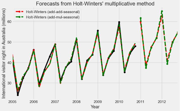
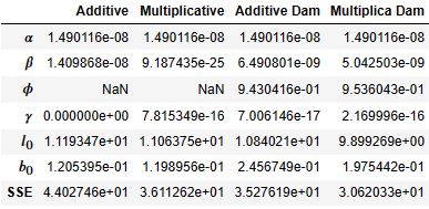
- Let’s examine the trend, slope, and seasonal components
fit1 = ExponentialSmoothing(
    aust,
    seasonal_periods=4,
    trend="add",
    seasonal="add",
    initialization_method="estimated",
).fit()
fit2 = ExponentialSmoothing(
    aust,
    seasonal_periods=4,
    trend="add",
    seasonal="mul",
    initialization_method="estimated",
).fit()
    columns=[r"$y_t$", r"$l_t$", r"$b_t$", r"$s_t$", r"$\hat{y}_t$"],

df = pd.DataFrame(
    np.c_[aust, fit2.level, fit2.trend, fit2.season, fit2.fittedvalues],
    columns=[r"$y_t$", r"$l_t$", r"$b_t$", r"$s_t$", r"$\hat{y}_t$"],
    index=aust.index,
)
forecasts = fit2.forecast(8).rename(r"$\hat{y}_t$").to_frame()
df = pd.concat([df, forecasts], axis=0, sort=True)

states1 = pd.DataFrame(
    np.c_[fit1.level, fit1.trend, fit1.season],
    columns=["level", "slope", "seasonal"],
    index=aust.index,
)
states2 = pd.DataFrame(
    np.c_[fit2.level, fit2.trend, fit2.season],
    columns=["level", "slope", "seasonal"],
    index=aust.index,
)
fig, [[ax1, ax4], [ax2, ax5], [ax3, ax6]] = plt.subplots(3, 2, figsize=(12, 8))
states1[["level"]].plot(ax=ax1)
states1[["slope"]].plot(ax=ax2)
states1[["seasonal"]].plot(ax=ax3)
states2[["level"]].plot(ax=ax4)
states2[["slope"]].plot(ax=ax5)
states2[["seasonal"]].plot(ax=ax6)
plt.show()
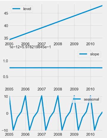
- Let’s look at forecasts and simulations from the Holt-Winters’ multiplicative method
fit = ExponentialSmoothing(
    aust,
    seasonal_periods=4,
    trend="add",
    seasonal="mul",
    initialization_method="estimated",
).fit()
simulations = fit.simulate(8, repetitions=100, error="mul")

ax = aust.plot(
    figsize=(10, 6),
    marker="o",
    color="black",
    title="Forecasts and simulations from Holt-Winters' multiplicative method",
)
ax.set_ylabel("International visitor night in Australia (millions)")
ax.set_xlabel("Year")
fit.fittedvalues.plot(ax=ax, style="--", color="green")
simulations.plot(ax=ax, style="-", alpha=0.05, color="grey", legend=False)
fit.forecast(8).rename("Holt-Winters (add-mul-seasonal)").plot(
    ax=ax, style="--", marker="o", color="green", legend=True
)
plt.show()
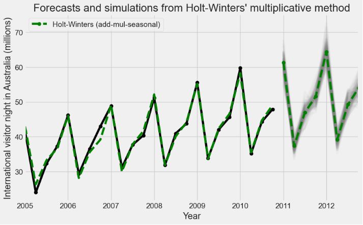
- Let’s run forecasts and simulations from the Holt-Winters’ multiplicative method with anchor=”2009-01-01″
fit = ExponentialSmoothing(
    aust,
    seasonal_periods=4,
    trend="add",
    seasonal="mul",
    initialization_method="estimated",
).fit()
simulations = fit.simulate(
    16, anchor="2009-01-01", repetitions=100, error="mul", random_errors="bootstrap"
)

ax = aust.plot(
    figsize=(10, 6),
    marker="o",
    color="black",
    title="Forecasts and simulations from Holt-Winters' multiplicative method",
)
ax.set_ylabel("International visitor night in Australia (millions)")
ax.set_xlabel("Year")
fit.fittedvalues.plot(ax=ax, style="--", color="green")
simulations.plot(ax=ax, style="-", alpha=0.05, color="grey", legend=False)
fit.forecast(8).rename("Holt-Winters (add-mul-seasonal)").plot(
    ax=ax, style="--", marker="o", color="green", legend=True
)
plt.show()
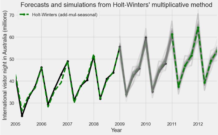
Hourly Energy Demand Forecasting
- This section addresses a multi-variable TSF problem to predict the next 24 hours of energy demand in Spain.
- The input Kaggle dataset contains 4 years of electrical consumption, generation, pricing, and weather data for Spain. Consumption and generation data was retrieved from ENTSOE a public portal for Transmission Service Operator (TSO) data. Settlement prices were obtained from the Spanish TSO Red Electric España. Weather data was purchased as part of a personal project from the Open Weather API for the 5 largest cities in Spain and made public here.
- Importing the key libraries, preparing the input data, and running the baseline multivariate TSF
import pandas as pd
import numpy as np
import matplotlib.pyplot as plt
import tensorflow as tf
from sklearn.preprocessing import MinMaxScaler
def load_data(col=None, path="energy_dataset.csv", verbose=False):
    df = pd.read_csv(path)
    if col is not None:
        df = df[col]
    if verbose:
        print(df.head())
    return df

print("Multivariate Sample")
multivar_df = load_data(['time','total load actual', 'price actual'], verbose=True)
Multivariate Sample
                         time  total load actual  price actual
0   2015-01-01 00:00:00+01:00            25385.0         65.41
1   2015-01-01 01:00:00+01:00            24382.0         64.92
..                        ...                ...           ...
3   2015-01-01 03:00:00+01:00            21286.0         59.32
4   2015-01-01 04:00:00+01:00            20264.0         56.04

[5 rows x 3 columns]
df = load_data(col=["total load forecast","total load actual"])

#fill nans with linear interpolation because this is how we will fill when using the data in the models.
df_filled = df.interpolate("linear")
mm = MinMaxScaler()
df_scaled = mm.fit_transform(df_filled)

df_prep = pd.DataFrame(df_scaled, columns=df.columns)
y_true = df_prep["total load actual"]
y_pred_forecast = df_prep["total load forecast"]

### persistence 1 day
#shift series by 24 hours
# realign y_true to have the same length and time samples
y_preds_persistance_1_day = y_true.shift(24).dropna()
persistence_1_day_mae = tf.keras.losses.MAE(y_true[y_preds_persistance_1_day.index], y_preds_persistance_1_day).numpy()
persistence_1_day_mape = tf.keras.losses.MAPE(np.maximum(y_true[y_preds_persistance_1_day.index], 1e-5), np.maximum(y_preds_persistance_1_day, 1e-5)).numpy()


### persistence 3 day average
#shift by 1, 2, 3 days. Realign to have same lengths. Average days and calcualte MAE.

shift_dfs = list()
for i in range(1, 4):
    shift_dfs.append(pd.Series(y_true.shift(24 * i), name=f"d{i}"))

y_persistance_3d = pd.concat(shift_dfs, axis=1).dropna()
y_persistance_3d["avg"] = (y_persistance_3d["d1"] + y_persistance_3d["d2"] + y_persistance_3d["d3"])/3
d3_idx = y_persistance_3d.index
persistence_3day_avg_mae = tf.keras.losses.MAE(y_true[d3_idx], y_persistance_3d['avg']).numpy()
persistence_3day_avg_mape = tf.keras.losses.MAPE(np.maximum(y_true[d3_idx], 1e-5), np.maximum(y_persistance_3d['avg'], 1e-5)).numpy()


ref_error = pd.DataFrame({
    "Method": ["TSO Forecast", "Persistence 1 Day", "Persitence 3 Day Avg"],
    "MAE": [tf.keras.losses.MAE(y_true, y_pred_forecast).numpy(),
            persistence_1_day_mae,
            persistence_3day_avg_mae],
    "MAPE":[tf.keras.losses.MAPE(np.maximum(y_true, 1e-5), np.maximum(y_pred_forecast, 1e-5)).numpy(),
            persistence_1_day_mape,
            persistence_3day_avg_mape]},
    index=[i for i in range(3)])

print("\nSummary of Baseline Errors")
print(ref_error)
print(f"\nAverage error in MW for TSO Forecast {round(df['total load forecast'].mean()*ref_error.iloc[0,1], 2)}")
Summary of Baseline Errors
                 Method       MAE       MAPE
0          TSO Forecast  0.015456   5.472781
1     Persistence 1 Day  0.106903  65.951647
2  Persitence 3 Day Avg  0.115176  84.151898

Average error in MW for TSO Forecast 443.76
- Preparing the input data for training the Deep Learning (DL) models
def clean_data(series):
    """Fills missing values.

        Interpolate missing values with a linear approximation.
    """
    series_filled = series.interpolate(method='linear')

    return series_filled


def min_max_scale(dataframe):
    """ Applies MinMax Scaling

        Wrapper for sklearn's MinMaxScaler class.
    """
    mm = MinMaxScaler()
    return mm.fit_transform(dataframe)

def make_time_features(series):

    #convert series to datetimes
    times = series.apply(lambda x: x.split('+')[0])
    datetimes = pd.DatetimeIndex(times)

    hours = datetimes.hour.values
    day = datetimes.dayofweek.values
    months = datetimes.month.values

    hour = pd.Series(hours, name='hours')
    dayofw = pd.Series(day, name='dayofw')
    month = pd.Series(months, name='months')

    return hour, dayofw, month

hour, day, month = make_time_features(multivar_df.time)
print("Hours")
print(hour.head())
print("Day of Week")
print(day.head())
print("Months")
print(month.head())

Hours
0    0
1    1
    ..
3    3
4    4
Name: hours, Length: 5, dtype: int32
Day of Week
0    3
1    3
    ..
3    3
4    3
Name: dayofw, Length: 5, dtype: int32
Months
0    1
1    1
    ..
3    1
4    1
Name: months, Length: 5, dtype: int32

def split_data(series, train_fraq, test_len=8760):
    """Splits input series into train, val and test.

        Default to 1 year of test data.
    """
    #slice the last year of data for testing 1 year has 8760 hours
    test_slice = len(series)-test_len

    test_data = series[test_slice:]
    train_val_data = series[:test_slice]

    #make train and validation from the remaining
    train_size = int(len(train_val_data) * train_fraq)

    train_data = train_val_data[:train_size]
    val_data = train_val_data[train_size:]

    return train_data, val_data, test_data


multivar_df = clean_data(multivar_df)

#add hour and month features
hours, day, months = make_time_features(multivar_df.time)
multivar_df = pd.concat([multivar_df.drop(['time'], axis=1), hours, day, months], axis=1)

#scale
multivar_df = min_max_scale(multivar_df)
train_multi, val_multi, test_multi = split_data(multivar_df, train_fraq=0.65, test_len=8760)
print("Multivarate Datasets")
print(f"Train Data Shape: {train_multi.shape}")
print(f"Val Data Shape: {val_multi.shape}")
print(f"Test Data Shape: {test_multi.shape}")
print(f"Nulls In Train {np.any(np.isnan(train_multi))}")
print(f"Nulls In Validation {np.any(np.isnan(val_multi))}")
print(f"Nulls In Test {np.any(np.isnan(test_multi))}")

Multivarate Datasets
Train Data Shape: (17097, 5)
Val Data Shape: (9207, 5)
Test Data Shape: (8760, 5)
Nulls In Train False
Nulls In Validation False
Nulls In Test False
def window_dataset(data, n_steps, n_horizon, batch_size, shuffle_buffer, multi_var=False, expand_dims=False):
    """ Create a windowed tensorflow dataset

    """

    #create a window with n steps back plus the size of the prediction length
    window = n_steps + n_horizon

    #expand dimensions to 3D to fit with LSTM inputs
    #creat the inital tensor dataset
    if expand_dims:
        ds = tf.expand_dims(data, axis=-1)
        ds = tf.data.Dataset.from_tensor_slices(ds)
    else:
        ds = tf.data.Dataset.from_tensor_slices(data)

    #create the window function shifting the data by the prediction length
    ds = ds.window(window, shift=n_horizon, drop_remainder=True)

    #flatten the dataset and batch into the window size
    ds = ds.flat_map(lambda x : x.batch(window))
    ds = ds.shuffle(shuffle_buffer)

    #create the supervised learning problem x and y and batch
    if multi_var:
        ds = ds.map(lambda x : (x[:-n_horizon], x[-n_horizon:, :1]))
    else:
        ds = ds.map(lambda x : (x[:-n_horizon], x[-n_horizon:]))

    ds = ds.batch(batch_size).prefetch(1)

    return ds

tf.random.set_seed(42)

n_steps = 72
n_horizon = 24
batch_size = 1
shuffle_buffer = 100


ds = window_dataset(train_multi, n_steps, n_horizon, batch_size, shuffle_buffer, multi_var=True)

print('Example sample shapes')
for idx,(x,y) in enumerate(ds):
    print("x = ", x.numpy().shape)
    print("y = ", y.numpy().shape)
    break

Example sample shapes
x =  (1, 72, 5)
y =  (1, 24, 1)

def build_dataset(train_fraq=0.65,
                  n_steps=24*30,
                  n_horizon=24,
                  batch_size=256,
                  shuffle_buffer=500,
                  expand_dims=False,
                  multi_var=False):
    """If multi variate then first column is always the column from which the target is contstructed.
    """

    tf.random.set_seed(23)

    if multi_var:
        data = load_data(col=['time', 'total load actual', 'price actual'])
        hours, day, months = make_time_features(data.time)
        data = pd.concat([data.drop(['time'], axis=1), hours, day, months], axis=1)
    else:
        data = load_data(col=['total load actual'])

    data = clean_data(data)

    if multi_var:
        mm = MinMaxScaler()
        data = mm.fit_transform(data)

    train_data, val_data, test_data = split_data(data, train_fraq=train_fraq, test_len=8760)

    train_ds = window_dataset(train_data, n_steps, n_horizon, batch_size, shuffle_buffer, multi_var=multi_var, expand_dims=expand_dims)
    val_ds = window_dataset(val_data, n_steps, n_horizon, batch_size, shuffle_buffer, multi_var=multi_var, expand_dims=expand_dims)
    test_ds = window_dataset(test_data, n_steps, n_horizon, batch_size, shuffle_buffer, multi_var=multi_var, expand_dims=expand_dims)


    print(f"Prediction lookback (n_steps): {n_steps}")
    print(f"Prediction horizon (n_horizon): {n_horizon}")
    print(f"Batch Size: {batch_size}")
    print("Datasets:")
    print(train_ds.element_spec)

    return train_ds, val_ds, test_ds

train_ds, val_ds, test_ds = build_dataset(multi_var=True)

Prediction lookback (n_steps): 720
Prediction horizon (n_horizon): 24
Batch Size: 256
Datasets:
(TensorSpec(shape=(None, None, 5), dtype=tf.float64, name=None), TensorSpec(shape=(None, None, 1), dtype=tf.float64, name=None))
- Training multiple DL models
- DNN model
def get_params(multivar=False):
    lr = 3e-4
    n_steps=24*30
    n_horizon=24
    if multivar:
        n_features=5
    else:
        n_features=1

    return n_steps, n_horizon, n_features, lr

model_configs = dict()

def cfg_model_run(model, history, test_ds):
    return {"model": model, "history" : history, "test_ds": test_ds}


def run_model(model_name, model_func, model_configs, epochs):

    n_steps, n_horizon, n_features, lr = get_params(multivar=True)
    train_ds, val_ds, test_ds = build_dataset(n_steps=n_steps, n_horizon=n_horizon, multi_var=True)

    model = model_func(n_steps, n_horizon, n_features, lr=lr)

    model_hist = model.fit(train_ds, validation_data=val_ds, epochs=epochs)

    model_configs[model_name] = cfg_model_run(model, model_hist, test_ds)
    return test_ds

def dnn_model(n_steps, n_horizon, n_features, lr):
    tf.keras.backend.clear_session()

    model = tf.keras.models.Sequential([
        tf.keras.layers.Flatten(input_shape=(n_steps, n_features)),
        tf.keras.layers.Dense(128, activation='relu'),
        tf.keras.layers.Dropout(0.3),
        tf.keras.layers.Dense(128, activation='relu'),
        tf.keras.layers.Dropout(0.3),
        tf.keras.layers.Dense(n_horizon)
    ], name='dnn')

    loss=tf.keras.losses.Huber()
    optimizer = tf.keras.optimizers.legacy.Adam(learning_rate=lr)


    model.compile(loss=loss, optimizer='adam', metrics=['mae'])

    return model


dnn = dnn_model(*get_params(multivar=True))
dnn.summary()

Model: "dnn"
_________________________________________________________________
 Layer (type)                Output Shape              Param #
=================================================================
 flatten (Flatten)           (None, 3600)              0

 dense (Dense)               (None, 128)               460928

 dropout (Dropout)           (None, 128)               0

 dense_1 (Dense)             (None, 128)               16512

 dropout_1 (Dropout)         (None, 128)               0

 dense_2 (Dense)             (None, 24)                3096

=================================================================
Total params: 480536 (1.83 MB)
Trainable params: 480536 (1.83 MB)
Non-trainable params: 0 (0.00 Byte)
- CNN model
def cnn_model(n_steps, n_horizon, n_features, lr=3e-4):

    tf.keras.backend.clear_session()

    model = tf.keras.models.Sequential([
        tf.keras.layers.Conv1D(64, kernel_size=6, activation='relu', input_shape=(n_steps,n_features)),
        tf.keras.layers.MaxPooling1D(2),
        tf.keras.layers.Conv1D(64, kernel_size=3, activation='relu'),
        tf.keras.layers.MaxPooling1D(2),
        tf.keras.layers.Flatten(),
        tf.keras.layers.Dropout(0.3),
        tf.keras.layers.Dense(128),
        tf.keras.layers.Dropout(0.3),
        tf.keras.layers.Dense(n_horizon)
    ], name="CNN")

    loss= tf.keras.losses.Huber()
    optimizer = tf.keras.optimizers.legacy.Adam(learning_rate=lr)

    model.compile(loss=loss, optimizer='adam', metrics=['mae'])

    return model

cnn = cnn_model(*get_params(multivar=True))
cnn.summary()

Model: "CNN"
_________________________________________________________________
 Layer (type)                Output Shape              Param #
=================================================================
 conv1d (Conv1D)             (None, 715, 64)           1984

 max_pooling1d (MaxPooling1  (None, 357, 64)           0
 D)

 conv1d_1 (Conv1D)           (None, 355, 64)           12352

 max_pooling1d_1 (MaxPoolin  (None, 177, 64)           0
 g1D)

 flatten (Flatten)           (None, 11328)             0

 dropout (Dropout)           (None, 11328)             0

 dense (Dense)               (None, 128)               1450112

 dropout_1 (Dropout)         (None, 128)               0

 dense_1 (Dense)             (None, 24)                3096

=================================================================
Total params: 1467544 (5.60 MB)
Trainable params: 1467544 (5.60 MB)
Non-trainable params: 0 (0.00 Byte)
_________________________________________________________________
- LSTM model
def lstm_model(n_steps, n_horizon, n_features, lr):

    tf.keras.backend.clear_session()

    model = tf.keras.models.Sequential([
        tf.keras.layers.LSTM(72, activation='relu', input_shape=(n_steps, n_features), return_sequences=True),
        tf.keras.layers.LSTM(48, activation='relu', return_sequences=False),
        tf.keras.layers.Flatten(),
        tf.keras.layers.Dropout(0.3),
        tf.keras.layers.Dense(128, activation='relu'),
        tf.keras.layers.Dropout(0.3),
        tf.keras.layers.Dense(n_horizon)
    ], name='lstm')

    loss = tf.keras.losses.Huber()
    optimizer = tf.keras.optimizers.legacy.Adam(learning_rate=lr)

    model.compile(loss=loss, optimizer='adam', metrics=['mae'])

    return model

lstm = lstm_model(*get_params(multivar=True))
lstm.summary()
Model: "lstm"
_________________________________________________________________
 Layer (type)                Output Shape              Param #
=================================================================
 lstm (LSTM)                 (None, 720, 72)           22464

 lstm_1 (LSTM)               (None, 48)                23232

 flatten (Flatten)           (None, 48)                0

 dropout (Dropout)           (None, 48)                0

 dense (Dense)               (None, 128)               6272

 dropout_1 (Dropout)         (None, 128)               0

 dense_1 (Dense)             (None, 24)                3096

=================================================================
Total params: 55064 (215.09 KB)
Trainable params: 55064 (215.09 KB)
Non-trainable params: 0 (0.00 Byte)
_________________________________________________________________
- LSTM CNN model
def lstm_cnn_model(n_steps, n_horizon, n_features, lr):

    tf.keras.backend.clear_session()

    model = tf.keras.models.Sequential([
        tf.keras.layers.Conv1D(64, kernel_size=6, activation='relu', input_shape=(n_steps,n_features)),
        tf.keras.layers.MaxPooling1D(2),
        tf.keras.layers.Conv1D(64, kernel_size=3, activation='relu'),
        tf.keras.layers.MaxPooling1D(2),
        tf.keras.layers.LSTM(72, activation='relu', return_sequences=True),
        tf.keras.layers.LSTM(48, activation='relu', return_sequences=False),
        tf.keras.layers.Flatten(),
        tf.keras.layers.Dropout(0.3),
        tf.keras.layers.Dense(128),
        tf.keras.layers.Dropout(0.3),
        tf.keras.layers.Dense(n_horizon)
    ], name="lstm_cnn")

    loss = tf.keras.losses.Huber()
    optimizer = tf.keras.optimizers.legacy.Adam(learning_rate=lr)

    model.compile(loss=loss, optimizer='adam', metrics=['mae'])

    return model

lstm_cnn = lstm_cnn_model(*get_params(multivar=True))
lstm_cnn.summary()
Model: "lstm_cnn"
_________________________________________________________________
 Layer (type)                Output Shape              Param #
=================================================================
 conv1d (Conv1D)             (None, 715, 64)           1984

 max_pooling1d (MaxPooling1  (None, 357, 64)           0
 D)

 conv1d_1 (Conv1D)           (None, 355, 64)           12352

 max_pooling1d_1 (MaxPoolin  (None, 177, 64)           0
 g1D)

 lstm (LSTM)                 (None, 177, 72)           39456

 lstm_1 (LSTM)               (None, 48)                23232

 flatten (Flatten)           (None, 48)                0

 dropout (Dropout)           (None, 48)                0

 dense (Dense)               (None, 128)               6272

 dropout_1 (Dropout)         (None, 128)               0

 dense_1 (Dense)             (None, 24)                3096

=================================================================
Total params: 86392 (337.47 KB)
Trainable params: 86392 (337.47 KB)
Non-trainable params: 0 (0.00 Byte)
_________________________________________________________________
- LSTM CNN skip model
def lstm_cnn_skip_model(n_steps, n_horizon, n_features, lr):

    tf.keras.backend.clear_session()


    inputs = tf.keras.layers.Input(shape=(n_steps,n_features), name='main')

    conv1 = tf.keras.layers.Conv1D(64, kernel_size=6, activation='relu')(inputs)
    max_pool_1 = tf.keras.layers.MaxPooling1D(2)(conv1)
    conv2 = tf.keras.layers.Conv1D(64, kernel_size=3, activation='relu')(max_pool_1)
    max_pool_2 = tf.keras.layers.MaxPooling1D(2)(conv2)
    lstm_1 = tf.keras.layers.LSTM(72, activation='relu', return_sequences=True)(max_pool_2)
    lstm_2 = tf.keras.layers.LSTM(48, activation='relu', return_sequences=False)(lstm_1)
    flatten = tf.keras.layers.Flatten()(lstm_2)

    skip_flatten = tf.keras.layers.Flatten()(inputs)

    concat = tf.keras.layers.Concatenate(axis=-1)([flatten, skip_flatten])
    drop_1 = tf.keras.layers.Dropout(0.3)(concat)
    dense_1 = tf.keras.layers.Dense(128, activation='relu')(drop_1)
    drop_2 = tf.keras.layers.Dropout(0.3)(dense_1)
    output = tf.keras.layers.Dense(n_horizon)(drop_2)

    model = tf.keras.Model(inputs=inputs, outputs=output, name='lstm_skip')

    loss = tf.keras.losses.Huber()
    optimizer = tf.keras.optimizers.Adam(learning_rate=lr)

    model.compile(loss=loss, optimizer='adam', metrics=['mae'])

    return model

lstm_skip = lstm_cnn_skip_model(*get_params(multivar=True))
lstm_skip.summary()
Model: "lstm_skip"
__________________________________________________________________________________________________
 Layer (type)                Output Shape                 Param #   Connected to
==================================================================================================
 main (InputLayer)           [(None, 720, 5)]             0         []

 conv1d (Conv1D)             (None, 715, 64)              1984      ['main[0][0]']

 max_pooling1d (MaxPooling1  (None, 357, 64)              0         ['conv1d[0][0]']
 D)

 conv1d_1 (Conv1D)           (None, 355, 64)              12352     ['max_pooling1d[0][0]']

 max_pooling1d_1 (MaxPoolin  (None, 177, 64)              0         ['conv1d_1[0][0]']
 g1D)

 lstm (LSTM)                 (None, 177, 72)              39456     ['max_pooling1d_1[0][0]']

 lstm_1 (LSTM)               (None, 48)                   23232     ['lstm[0][0]']

 flatten (Flatten)           (None, 48)                   0         ['lstm_1[0][0]']

 flatten_1 (Flatten)         (None, 3600)                 0         ['main[0][0]']

 concatenate (Concatenate)   (None, 3648)                 0         ['flatten[0][0]',
                                                                     'flatten_1[0][0]']

 dropout (Dropout)           (None, 3648)                 0         ['concatenate[0][0]']

 dense (Dense)               (None, 128)                  467072    ['dropout[0][0]']

 dropout_1 (Dropout)         (None, 128)                  0         ['dense[0][0]']

 dense_1 (Dense)             (None, 24)                   3096      ['dropout_1[0][0]']

==================================================================================================
Total params: 547192 (2.09 MB)
Trainable params: 547192 (2.09 MB)
Non-trainable params: 0 (0.00 Byte)
__________________________________________________________________________________________________
- Training the hybrid DL model
model_configs=dict()
run_model("dnn", dnn_model, model_configs, epochs=50)
run_model("cnn", cnn_model, model_configs, epochs=50)
run_model("lstm", lstm_model, model_configs, epochs=50)
run_model("lstm_cnn", lstm_cnn_model, model_configs, epochs=50)
run_model("lstm_skip", lstm_cnn_skip_model, model_configs, epochs=50)
Prediction lookback (n_steps): 720
Prediction horizon (n_horizon): 24
Batch Size: 256
Datasets:
(TensorSpec(shape=(None, None, 5), dtype=tf.float64, name=None), TensorSpec(shape=(None, None, 1), dtype=tf.float64, name=None))
Epoch 1/50
3/3 [==============================] - 1s 168ms/step - loss: 0.3135 - mae: 0.6585 - val_loss: 0.1146 - val_mae: 0.3994
..................
Epoch 49/50
3/3 [==============================] - 2s 540ms/step - loss: 0.0345 - mae: 0.2050 - val_loss: 0.0410 - val_mae: 0.2296
Epoch 50/50
3/3 [==============================] - 2s 510ms/step - loss: 0.0329 - mae: 0.1995 - val_loss: 0.0391 - val_mae: 0.2247
- Plotting Loss Curves
legend = list()

fig, axs = plt.subplots(1, 5, figsize=(15,5))

def plot_graphs(metric, val, ax, upper):
    ax.plot(val['history'].history[metric])
    ax.plot(val['history'].history[f'val_{metric}'])
    ax.set_title(key)
    ax.legend([metric, f"val_{metric}"])
    ax.set_xlabel('epochs')
    ax.set_ylabel(metric)
    ax.set_ylim([0, upper])

for (key, val), ax in zip(model_configs.items(), axs.flatten()):
    plot_graphs('loss', val, ax, 0.2)
print("Loss Curves")
Loss Curves
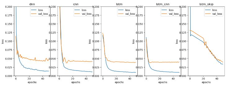
- Plotting MAE curves
print("MAE Curves")
fig, axs = plt.subplots(1, 5, figsize=(15,5))
for (key, val), ax in zip(model_configs.items(), axs.flatten()):
    plot_graphs('mae', val, ax, 0.6)
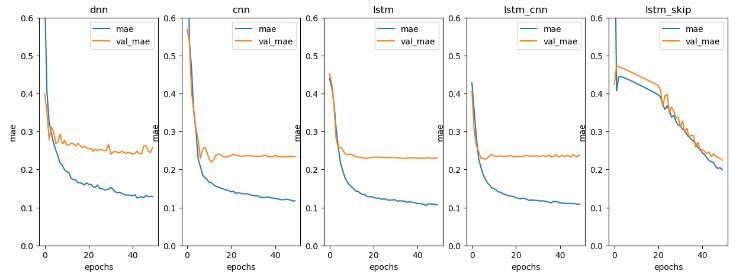
- DL performance summary
names = list()
performance = list()

for key, value in model_configs.items():
    names.append(key)
    mae = value['model'].evaluate(value['test_ds'])
    performance.append(mae[1])

performance_df = pd.DataFrame(performance, index=names, columns=['mae'])
performance_df['error_mw'] = performance_df['mae'] * df['total load forecast'].mean()
print(performance_df)
2/2 [==============================] - 0s 9ms/step - loss: 0.0068 - mae: 0.0874
2/2 [==============================] - 0s 17ms/step - loss: 0.0079 - mae: 0.0945
2/2 [==============================] - 1s 161ms/step - loss: 0.0077 - mae: 0.0971
2/2 [==============================] - 0s 55ms/step - loss: 0.0079 - mae: 0.0980
2/2 [==============================] - 0s 52ms/step - loss: 0.0179 - mae: 0.1424
                mae     error_mw
dnn        0.087427  2510.221097
cnn        0.094523  2713.965580
...             ...          ...
lstm_cnn   0.097980  2813.224550
lstm_skip  0.142392  4088.364191

[5 rows x 2 columns]
- Plotting actual data vs First 2 Weeks of Predictions
fig, axs = plt.subplots(5, 1, figsize=(14, 10))
days = 14

vline = np.linspace(0, days*24, days+1)

for (key, val), ax in zip(model_configs.items(), axs):

    test = val['test_ds']
    preds = val['model'].predict(test)

    xbatch, ybatch = iter(test).get_next()

    ax.plot(ybatch.numpy()[:days].reshape(-1))
    ax.plot(preds[:days].reshape(-1))
    ax.set_title(key)
    ax.vlines(vline, ymin=0, ymax=1, linestyle='dotted', transform = ax.get_xaxis_transform())
    ax.legend(["Actual", "Predicted"],loc='lower left')

plt.xlabel("Hours Cumulative")
print('First Two Weeks of Predictions')

2/2 [==============================] - 0s 6ms/step
2/2 [==============================] - 0s 11ms/step
2/2 [==============================] - 1s 143ms/step
2/2 [==============================] - 0s 50ms/step
2/2 [==============================] - 0s 54ms/step
First Two Weeks of Predictions
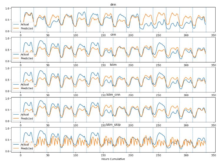
- Read more here.
Stock Price Forecasting – 1. TSLA
- Let’s turn our attention to the ML-based TSF of TSLA prices 2020-2023 using RNN in TensorFlow.
- Importing the key libraries and input data
import numpy as np
import pandas as pd
import yfinance as yf
import datetime as dt
import matplotlib.pyplot as plt
import math
#the start and end date
start_date = dt.datetime(2020,1,1)
end_date = dt.datetime(2023,12,15)

#loading from yahoo finance
data = yf.download("TSLA",start_date, end_date)

pd.set_option('display.max_rows', 4)
pd.set_option('display.max_columns',5)
print(data)
[*********************100%%**********************]  1 of 1 completed
                  Open        High  ...   Adj Close     Volume
Date                                ...
2020-01-02   28.299999   28.713333  ...   28.684000  142981500
2020-01-03   29.366667   30.266666  ...   29.534000  266677500
...                ...         ...  ...         ...        ...
2023-12-13  234.190002  240.300003  ...  239.289993  145825100
2023-12-14  241.220001  248.009995  ...  246.884995   36237310

[996 rows x 6 columns]
- Splitting the dataset and setting 70 % data for training
# Setting 70 percent data for training
training_data_len = math.ceil(len(data) * .7)
training_data_len

#Splitting the dataset
train_data = data[:training_data_len].iloc[:,:1]
test_data = data[training_data_len:].iloc[:,:1]
print(train_data.shape, test_data.shape)
(698, 1) (298, 1)

# Selecting Open Price values
dataset_train = train_data.Open.values
# Reshaping 1D to 2D array
dataset_train = np.reshape(dataset_train, (-1,1))
dataset_train.shape
(698, 1)
from sklearn.preprocessing import MinMaxScaler
scaler = MinMaxScaler(feature_range=(0,1))
# scaling dataset
scaled_train = scaler.fit_transform(dataset_train)

#print(scaled_train[:5])

# Selecting Open Price values
dataset_test = test_data.Open.values
# Reshaping 1D to 2D array
dataset_test = np.reshape(dataset_test, (-1,1))
# Normalizing values between 0 and 1
scaled_test = scaler.fit_transform(dataset_test)
#print(*scaled_test[:5])

X_train = []
y_train = []
for i in range(50, len(scaled_train)):
    X_train.append(scaled_train[i-50:i, 0])
    y_train.append(scaled_train[i, 0])
    if i <= 51:
#        print(X_train)
#        print(y_train)
#        print()

X_test = []
y_test = []
for i in range(50, len(scaled_test)):
    X_test.append(scaled_test[i-50:i, 0])
    y_test.append(scaled_test[i, 0])

# The data is converted to Numpy array
X_train, y_train = np.array(X_train), np.array(y_train)

#Reshaping
X_train = np.reshape(X_train, (X_train.shape[0], X_train.shape[1],1))
y_train = np.reshape(y_train, (y_train.shape[0],1))
print("X_train :",X_train.shape,"y_train :",y_train.shape)
X_train : (648, 50, 1) y_train : (648, 1)

# The data is converted to numpy array
X_test, y_test = np.array(X_test), np.array(y_test)

#Reshaping
X_test = np.reshape(X_test, (X_test.shape[0], X_test.shape[1],1))
y_test = np.reshape(y_test, (y_test.shape[0],1))
print("X_test :",X_test.shape,"y_test :",y_test.shape)
X_test : (248, 50, 1) y_test : (248, 1)
- Training the RNN model
!pip install tensorflow
# importing libraries
import tensorflow as tf
import keras
from keras.models import Sequential
from keras.layers import LSTM
from keras.layers import Dense
from keras.layers import SimpleRNN
from keras.layers import Dropout
from keras.layers import GRU, Bidirectional
from keras.optimizers import SGD
from sklearn import metrics
from sklearn.metrics import mean_squared_error
# initializing the RNN
regressor = Sequential()

# adding RNN layers and dropout regularization
regressor.add(SimpleRNN(units = 50,
                        activation = "tanh",
                        return_sequences = True,
                        input_shape = (X_train.shape[1],1)))
regressor.add(Dropout(0.2))

regressor.add(SimpleRNN(units = 50,
                        activation = "tanh",
                        return_sequences = True))

regressor.add(SimpleRNN(units = 50,
                        activation = "tanh",
                        return_sequences = True))

regressor.add( SimpleRNN(units = 50))

# adding the output layer
regressor.add(Dense(units = 1,activation='sigmoid'))

# compiling RNN
opt = tf.keras.optimizers.legacy.SGD(learning_rate=0.01, momentum=0.9)
regressor.compile(opt,
                  loss = "mean_squared_error")

# fitting the model
regressor.fit(X_train, y_train, epochs = 10, batch_size = 2)
regressor.summary()
Epoch 1/10
324/324 [==============================] - 7s 17ms/step - loss: 0.0116
Epoch 2/10
324/324 [==============================] - 6s 18ms/step - loss: 0.0037
Epoch 3/10
324/324 [==============================] - 6s 17ms/step - loss: 0.0041
Epoch 4/10
324/324 [==============================] - 6s 17ms/step - loss: 0.0028
Epoch 5/10
324/324 [==============================] - 6s 18ms/step - loss: 0.0028
Epoch 6/10
324/324 [==============================] - 6s 18ms/step - loss: 0.0024
Epoch 7/10
324/324 [==============================] - 6s 19ms/step - loss: 0.0027
Epoch 8/10
324/324 [==============================] - 6s 18ms/step - loss: 0.0021
Epoch 9/10
324/324 [==============================] - 6s 17ms/step - loss: 0.0021
Epoch 10/10
324/324 [==============================] - 6s 17ms/step - loss: 0.0020
Model: "sequential_5"
_________________________________________________________________
 Layer (type)                Output Shape              Param #
=================================================================
 simple_rnn_8 (SimpleRNN)    (None, 50, 50)            2600

 dropout_4 (Dropout)         (None, 50, 50)            0

 simple_rnn_9 (SimpleRNN)    (None, 50, 50)            5050

 simple_rnn_10 (SimpleRNN)   (None, 50, 50)            5050

 simple_rnn_11 (SimpleRNN)   (None, 50)                5050

 dense_6 (Dense)             (None, 1)                 51

=================================================================
Total params: 17801 (69.54 KB)
Trainable params: 17801 (69.54 KB)
Non-trainable params: 0 (0.00 Byte)
_________________________________________________________________
- Training the LSTM model
#Initialising the model
regressorLSTM = Sequential()

#Adding LSTM layers
regressorLSTM.add(LSTM(50,
                       return_sequences = True,
                       input_shape = (X_train.shape[1],1)))
regressorLSTM.add(LSTM(50,
                       return_sequences = False))
regressorLSTM.add(Dense(25))

#Adding the output layer
regressorLSTM.add(Dense(1))

#Compiling the model
regressorLSTM.compile(optimizer = 'adam',
                      loss = 'mean_squared_error',
                      metrics = ["accuracy"])

#Fitting the model
regressorLSTM.fit(X_train,
                  y_train,
                  batch_size = 1,
                  epochs = 12)
regressorLSTM.summary()

648/648 [==============================] - 10s 11ms/step - loss: 0.0061 - accuracy: 0.0031
Epoch 2/12
648/648 [==============================] - 7s 11ms/step - loss: 0.0029 - accuracy: 0.0031
Epoch 3/12
648/648 [==============================] - 7s 11ms/step - loss: 0.0021 - accuracy: 0.0031
Epoch 4/12
648/648 [==============================] - 7s 11ms/step - loss: 0.0016 - accuracy: 0.0031
Epoch 5/12
648/648 [==============================] - 7s 11ms/step - loss: 0.0015 - accuracy: 0.0031
Epoch 6/12
648/648 [==============================] - 8s 12ms/step - loss: 0.0014 - accuracy: 0.0031
Epoch 7/12
648/648 [==============================] - 7s 11ms/step - loss: 0.0012 - accuracy: 0.0031
Epoch 8/12
648/648 [==============================] - 7s 12ms/step - loss: 0.0013 - accuracy: 0.0031
Epoch 9/12
648/648 [==============================] - 7s 11ms/step - loss: 0.0011 - accuracy: 0.0031
Epoch 10/12
648/648 [==============================] - 7s 11ms/step - loss: 0.0010 - accuracy: 0.0031
Epoch 11/12
648/648 [==============================] - 7s 11ms/step - loss: 0.0010 - accuracy: 0.0031
Epoch 12/12
648/648 [==============================] - 8s 12ms/step - loss: 0.0011 - accuracy: 0.0031
Model: "sequential_2"
_________________________________________________________________
 Layer (type)                Output Shape              Param #
=================================================================
 lstm (LSTM)                 (None, 50, 50)            10400

 lstm_1 (LSTM)               (None, 50)                20200

 dense_2 (Dense)             (None, 25)                1275

 dense_3 (Dense)             (None, 1)                 26

=================================================================
Total params: 31901 (124.61 KB)
Trainable params: 31901 (124.61 KB)
Non-trainable params: 0 (0.00 Byte)
- Training the GRU model
#Initialising the model
regressorGRU = Sequential()

# GRU layers with Dropout regularisation
regressorGRU.add(GRU(units=50,
                     return_sequences=True,
                     input_shape=(X_train.shape[1],1),
                     activation='tanh'))
regressorGRU.add(Dropout(0.2))

regressorGRU.add(GRU(units=50,
                     return_sequences=True,
                     activation='tanh'))

regressorGRU.add(GRU(units=50,
                     return_sequences=True,
                     activation='tanh'))

regressorGRU.add(GRU(units=50,
                     activation='tanh'))

# The output layer
regressorGRU.add(Dense(units=1,
                       activation='relu'))
# Compiling the RNN
optgru = tf.keras.optimizers.legacy.SGD(learning_rate=0.1)
regressorGRU.compile(optimizer=optgru,
                     loss='mean_squared_error')

# Fitting the data
regressorGRU.fit(X_train,y_train,epochs=20,batch_size=1)
regressorGRU.summary()

648/648 [==============================] - 19s 24ms/step - loss: 0.0141
Epoch 2/20
648/648 [==============================] - 15s 23ms/step - loss: 0.0043
Epoch 3/20
648/648 [==============================] - 15s 23ms/step - loss: 0.0037
Epoch 4/20
648/648 [==============================] - 15s 23ms/step - loss: 0.0036
Epoch 5/20
648/648 [==============================] - 15s 23ms/step - loss: 0.0033
Epoch 6/20
648/648 [==============================] - 15s 23ms/step - loss: 0.0031
Epoch 7/20
648/648 [==============================] - 15s 23ms/step - loss: 0.0026
Epoch 8/20
648/648 [==============================] - 15s 23ms/step - loss: 0.0027
Epoch 9/20
648/648 [==============================] - 15s 23ms/step - loss: 0.0026
Epoch 10/20
648/648 [==============================] - 16s 24ms/step - loss: 0.0025
Epoch 11/20
648/648 [==============================] - 15s 23ms/step - loss: 0.0024
Epoch 12/20
648/648 [==============================] - 15s 24ms/step - loss: 0.0022
Epoch 13/20
648/648 [==============================] - 15s 24ms/step - loss: 0.0023
Epoch 14/20
648/648 [==============================] - 15s 23ms/step - loss: 0.0023
Epoch 15/20
648/648 [==============================] - 16s 24ms/step - loss: 0.0021
Epoch 16/20
648/648 [==============================] - 15s 23ms/step - loss: 0.0021
Epoch 17/20
648/648 [==============================] - 16s 25ms/step - loss: 0.0021
Epoch 18/20
648/648 [==============================] - 15s 23ms/step - loss: 0.0020
Epoch 19/20
648/648 [==============================] - 16s 24ms/step - loss: 0.0020
Epoch 20/20
648/648 [==============================] - 16s 24ms/step - loss: 0.0022
Model: "sequential_4"
_________________________________________________________________
 Layer (type)                Output Shape              Param #
=================================================================
 gru_4 (GRU)                 (None, 50, 50)            7950

 dropout_3 (Dropout)         (None, 50, 50)            0

 gru_5 (GRU)                 (None, 50, 50)            15300

 gru_6 (GRU)                 (None, 50, 50)            15300

 gru_7 (GRU)                 (None, 50)                15300

 dense_5 (Dense)             (None, 1)                 51

=================================================================
Total params: 53901 (210.55 KB)
Trainable params: 53901 (210.55 KB)
Non-trainable params: 0 (0.00 Byte)
- Deep Learning predictions with test data
# predictions with X_test data
y_RNN = regressor.predict(X_test)
y_LSTM = regressorLSTM.predict(X_test)
y_GRU = regressorGRU.predict(X_test)
8/8 [==============================] - 0s 6ms/step
8/8 [==============================] - 0s 7ms/step
8/8 [==============================] - 0s 13ms/step

# scaling back from 0-1 to original
y_RNN_O = scaler.inverse_transform(y_RNN)
y_LSTM_O = scaler.inverse_transform(y_LSTM)
y_GRU_O = scaler.inverse_transform(y_GRU)

fig, axs = plt.subplots(3,figsize =(10,6),sharex=True, sharey=True)
fig.suptitle('Model Predictions')

#Plot for RNN predictions
axs[0].plot(train_data.index[150:], train_data.Open[150:], label = "train_data", color = "b")
axs[0].plot(test_data.index, test_data.Open, label = "test_data", color = "g")
axs[0].plot(test_data.index[50:], y_RNN_O, label = "y_RNN", color = "brown")
axs[0].legend()
axs[0].title.set_text("Basic RNN")

#Plot for LSTM predictions
axs[1].plot(train_data.index[150:], train_data.Open[150:], label = "train_data", color = "b")
axs[1].plot(test_data.index, test_data.Open, label = "test_data", color = "g")
axs[1].plot(test_data.index[50:], y_LSTM_O, label = "y_LSTM", color = "orange")
axs[1].legend()
axs[1].title.set_text("LSTM")

#Plot for GRU predictions
axs[2].plot(train_data.index[150:], train_data.Open[150:], label = "train_data", color = "b")
axs[2].plot(test_data.index, test_data.Open, label = "test_data", color = "g")
axs[2].plot(test_data.index[50:], y_GRU_O, label = "y_GRU", color = "red")
axs[2].legend()
axs[2].title.set_text("GRU")

plt.xlabel("Days")
plt.ylabel("Open price")

plt.show()

Stock Price Forecasting – 2. KO
- Let’s predict the univariate KO stock price 2021-2023 using the FB Prophet algorithm (Read more about FB Prophet here).
- Importing the key libraries, reading the stock data, and plotting both Close price and 25-Day MA
end_date =  date.today().strftime("%Y-%m-%d")
start_date = '2021-01-01'

# Getting quotes
stockname = 'Coca Cola'
symbol = 'KO'

import yfinance as yf
df = yf.download(symbol, start=start_date, end=end_date)

# Quick overview of dataset
print(df.head())
[*********************100%%**********************]  1 of 1 completed
                 Open       High        Low      Close  Adj Close    Volume
Date
2021-01-04  54.270000  54.630001  52.029999  52.759998  48.158413  25611100
2021-01-05  52.330002  52.619999  52.029999  52.180000  47.629009  20323800
2021-01-06  51.970001  52.020000  50.189999  50.520000  46.113785  38724500
2021-01-07  50.090000  50.259998  49.520000  49.959999  45.602623  53225700
2021-01-08  50.029999  51.130001  49.840000  51.080002  46.624939  29674000

# Visualize the original time series
rolling_window=25
y_a_add_ma = df['Close'].rolling(window=rolling_window).mean()

fig, ax = plt.subplots(figsize=(14,6))
sns.set(font_scale=1.1)
sns.lineplot(data=df, x=df.index, y='Close', color='red', linewidth=2, label='Close')
sns.lineplot(data=df, x=df.index, y=y_a_add_ma,
    linewidth=2.0, color='blue', linestyle='--', label=f'{rolling_window}-Day MA')
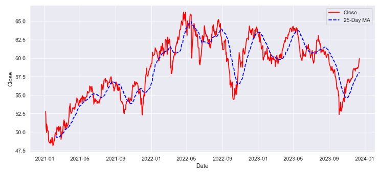
- Data preparation for Prophet
df_x = df[['Close']].copy()
df_x['ds'] = df.index.copy()
df_x.rename(columns={'Close': 'y'}, inplace=True)
df_x.reset_index(inplace=True, drop=True)
df_x.dropna(inplace=True)
df_x.tail(3)
           y	ds
739	59.040001	2023-12-11
740	59.419998	2023-12-12
741	59.930000	2023-12-13
- Fitting the Prophet model and generating the forecast
# This function fits the prophet model to the input data and generates a forecast
def fit_and_forecast(df, periods, interval_width, changepoint_range=0.8):

    # set the uncertainty interval
    Prophet(interval_width=interval_width)
    # Instantiate the model
    model = Prophet(changepoint_range=changepoint_range)

    # Fit the model
    model.fit(df)

    # Create a dataframe with a given number of dates
    future_df = model.make_future_dataframe(periods=periods)

    # Generate a forecast for the given dates
    forecast_df = model.predict(future_df)
    #print(forecast_df.head())
    return forecast_df, model, future_df


# Forecast for 365 days with full data
forecast_df, model, future_df = fit_and_forecast(df_x, 365, 0.95)
print(forecast_df.columns)
forecast_df[['yhat_lower', 'yhat_upper', 'yhat']].head(5)
Index(['ds', 'trend', 'yhat_lower', 'yhat_upper', 'trend_lower', 'trend_upper',
       'additive_terms', 'additive_terms_lower', 'additive_terms_upper',
       'weekly', 'weekly_lower', 'weekly_upper', 'yearly', 'yearly_lower',
       'yearly_upper', 'multiplicative_terms', 'multiplicative_terms_lower',
       'multiplicative_terms_upper', 'yhat'],
      dtype='object')
    yhat_lower	yhat_upper	yhat
0	49.414611	51.927240	50.635599
1	49.189039	51.795523	50.529285
2	49.244847	51.861979	50.514023
3	49.017967	51.661954	50.423064
4	49.134359	51.723404	50.444816
- Plotting the Prophet prediction
model.plot(forecast_df, uncertainty=True)

# Visualize the Forecast
def visualize_the_forecast(df_f, df_o):
    rolling_window = 20
    yhat_mean = df_f['yhat'].rolling(window=rolling_window).mean()

    # Thin out the ground truth data for illustration purposes
    df_lim = df_o
    # Print the Forecast
    fig, ax = plt.subplots(figsize=[14,7])
    sns.lineplot(data=df_f, x=df_f.ds, y=yhat_mean, ax=ax, label='predicted path', color='blue')
    sns.lineplot(data=df_lim, x=df_lim.ds, y='y', ax=ax, label='ground_truth', color='orange')
    #sns.lineplot(data=df_f, x=df_f.ds, y='yhat_lower', ax=ax, label='yhat_lower', color='skyblue', linewidth=1.0)
    #sns.lineplot(data=df_f, x=df_f.ds, y='yhat_upper', ax=ax, label='yhat_upper', color='coral', linewidth=1.0)
    plt.fill_between(df_f.ds, df_f.yhat_lower, df_f.yhat_upper, color='lightgreen')
    plt.legend(framealpha=0)
    ax.set(ylabel=stockname + " stock price")
    ax.set(xlabel=None)

visualize_the_forecast(forecast_df, df_x)
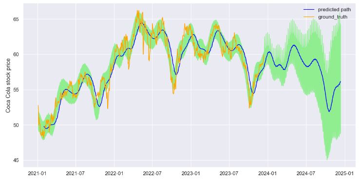
- Plotting the key components
model.plot_components(forecast_df, True, weekly_start=1)
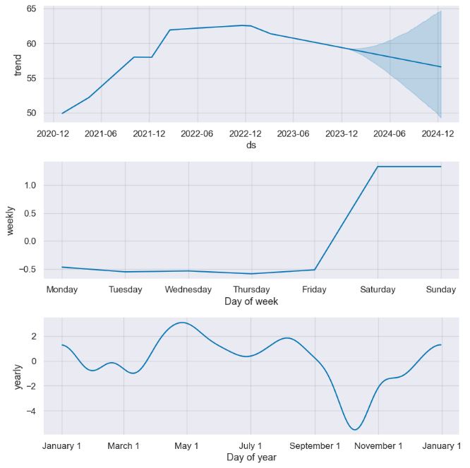
- Adjusting the Prophet change points to our model
# Printing the ChangePoints of our Model
forecast_df, model, future_df = fit_and_forecast(df_x, 365, 1.0)
axislist = add_changepoints_to_plot(model.plot(forecast_df).gca(), model, forecast_df)
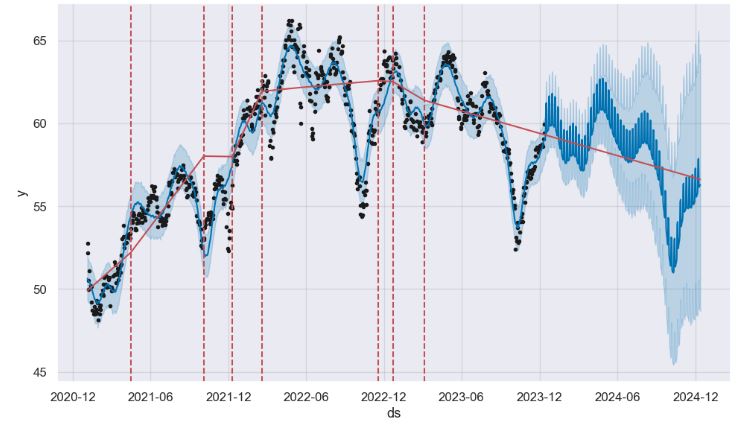
FinTech Sentiment Analysis
- In this section, we’ll use the stock sentiment analysis by using vader. The objective is to process the financial headlines by batch to generate an indicator of the market sentiment in real time.
- Importing the key libraries and defining the stock ticker
import pandas as pd
from datetime import datetime

from bs4 import BeautifulSoup
import nltk
from nltk.sentiment.vader import SentimentIntensityAnalyzer
import requests

# Define the ticker
tickers_list = ['KO']
- Reading the relevant financial headlines
news = pd.DataFrame()

for ticker in tickers_list:
   url = f'https://finviz.com/quote.ashx?t={ticker}&p=d'
   ret = requests.get(
       url,
       headers={'User-Agent': 'Mozilla/5.0 (Windows NT 10.0; Win64; x64) AppleWebKit/537.36 (KHTML, like Gecko) Chrome/111.0.0.0 Safari/537.36'},
   )

   html = BeautifulSoup(ret.content, "html.parser")

   try:
     df = pd.read_html(
         str(html),
         attrs={'class': 'fullview-news-outer'}
     )[0]
   except:
     print(f"{ticker} No news found")
     continue

   df.columns = ['Date', 'Headline']

df.tail()
       Date	           Headline
95	02:22AM	20 Highest Quality Vodkas in the World (Inside...
96	Dec-07-23 09:03PM	Uncover Warren Buffett's top 6 stocks for unri...
97	03:27PM	Campbell Soup CEO: How to lead successfully wi...
98	03:06PM	How To Earn $500 Per Month From Coca-Cola Stoc...
99	02:59PM	Coca-Cola partners with CustomerX.i to deliver...
- Data editing and NLP transformations
# Process date and time columns to make sure this is filled in every headline each row
dateNTime = df.Date.apply(lambda x: ','+x if len(x)<8 else x).str.split(r' |,', expand = True).replace("", None).ffill()
df = pd.merge(df, dateNTime, right_index=True, left_index=True).drop('Date', axis=1).rename(columns={0:'Date', 1:'Time'})
df = df[df["Headline"].str.contains("Loading.") == False].loc[:, ['Date', 'Time', 'Headline']]
df["Ticker"] = ticker
news = pd.concat([news, df], ignore_index = True)
nltk.download('vader_lexicon')
vader = SentimentIntensityAnalyzer()

scored_news = news.join(
  pd.DataFrame(news['Headline'].apply(vader.polarity_scores).tolist())
)
news.head()
    Date	Time	    Headline	             Ticker
0	Today	06:50AM	1 Warren Buffett Dow Jones Dividend Stock to B...	KO
1	Today	06:26AM	3 Safe Dividend Stocks to Buy in 2024 (Motley ...	KO
2	Today	05:49AM	Nearly 80% of Warren Buffett's Portfolio Is In...	KO
3	Today	05:23AM	Forget Coca-Cola. Here Are 2 Top Dividend Stoc...	KO
4	Jan-02-24	08:30AM	55% of Warren Buffett's $367 Billion Portfolio...	KO
- Plotting the KO sentiment score
news_score = scored_news.loc[:, ['Ticker', 'Date', 'compound']].pivot_table(values='compound', index='Date', columns='Ticker', aggfunc='mean').ewm(5).mean()
news_score.dropna().plot(figsize=(14, 5),linewidth=4,kind='line',legend=True, fontsize=14)
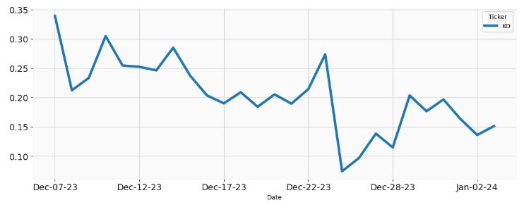
- Plotting the percentage change of the KO sentiment score
news_score.pct_change().dropna().plot(figsize=(14, 5),linewidth=4,kind='line',legend=True, fontsize=14)

Discussion
- We have investigated ways to circumvent the most common TSF errors:
- We checked our data for seasonal patterns and use appropriate methods to remove them, such as differencing, decomposition, or seasonal adjustment.
- Overfitting vs underfitting: We have to split our data into training and test sets and apply cross-validation or regularization on both.
- Most TSF models are based on certain assumptions about the data, such as stationarity, normality, linearity, or independence. We checked our data and model for any violations of the assumptions and apply appropriate transformations, tests, or corrections if needed.
- Forecasting is inherently uncertain. Therefore, it is important to quantify and communicate the uncertainty and probabilistic confidence of TSF.
- Time series forecasting models are dynamic. Therefore, it is important to monitor our model performance and compare it with the actual data in real time, and update/validate our model regularly.
- We need to define the business objectives of the forecast clearly, and choose the model and the methods that are appropriate and relevant for the decision making process.
- Key takeaways:
- High-quality data is essential for meaningful TSA
- Choosing the right model has a substantial impact on the quality of forecasts
- Identifying and modeling complex seasonality and trends can be a complex task, particularly when they evolve over time.
- Some time series data exhibits non-stationarity, where statistical properties change over time. Techniques like differencing or detrending may be needed to transform the data into a stationary form, facilitating more accurate modeling.
- Bottom line: We should communicate the forecast results and the assumptions/limitations of the underlying model effectively, and provide recommendations or actions based on the forecast.
Conclusions
- This study reviews a time-series-based approach for forecasting a sequence of data points collected over an interval of time.
- We have implemented an integrated TSF framework that uses a variety of statistical and ML-based methods. Statistical methods (seasonal decomposition, exponential smoothing, SARIMAX, etc.) typically involve modeling the underlying patterns and trends in the data, while supervised ML methods use regression algorithms to learn patterns and make predictions.
- The present approach includes comprehensive (X-) validation tests, null hypothesis testing, time-series QC diagnostics and prediction intervals to communicate uncertainty.
- We have analyzed the following business applications of TSF: macro-economics and fintech, meteorology, climate and environmental science (CO2 content, air pollution, etc.), sales data analysis and demand forecasting, stock price prediction, market sentiment analysis, and hourly energy consumption.
- Future TSF trends: IoT, multivariate big data, and cross-discipline applications.
Hands-On TSA(F) Tutorials
- Time series forecasting
- Sales Forecast Prediction – Python
- Public Python Tutorials
- 𝐓𝐢𝐦𝐞 𝐒𝐞𝐫𝐢𝐞𝐬 𝐀𝐧𝐚𝐥𝐲𝐬𝐢𝐬 𝐃𝐞𝐦𝐲𝐬𝐭𝐢𝐟𝐢𝐞𝐝: 𝐓𝐨𝐩 𝟐𝟎 𝐏𝐲𝐭𝐡𝐨𝐧 𝐋𝐢𝐛𝐫𝐚𝐫𝐢𝐞𝐬 𝐩𝐥𝐮𝐬 𝐓𝐲𝐩𝐞𝐬, 𝐀𝐩𝐩𝐥𝐢𝐜𝐚𝐭𝐢𝐨𝐧𝐬 𝐚𝐧𝐝 𝐅𝐮𝐧𝐜𝐭𝐢𝐨𝐧𝐬
- Sales Prediction Using Machine Learning
- Forecasting Future Sales Using Machine Learning
- Time Series Part 3: Forecasting with Facebook Prophet: An Intro
- Understanding FB Prophet: A Time Series Forecasting Algorithm
- A Comprehensive Beginner’s Guide to Creating a Time Series Forecast (With Codes in Python and R)
- CO2 Emission Forecast with Python (Seasonal ARIMA)
- What are the most common time series forecasting errors and how can you avoid them?
- Basics of Time Series Analysis and Its Application to Forecasting
Explore More
- Real-Time Stock Sentiment Analysis w/ NLP Web Scraping
- Evaluation of ML Sales Forecasting: tslearn, Random Walk, Holt-Winters, SARIMAX, GARCH, Prophet, and LSTM
- Real-Time Anomaly Detection of NAB Ambient Temperature Readings using the TensorFlow/Keras Autoencoder
- Time Series Forecasting of Hourly U.S.A. Energy Consumption – PJM East Electricity Grid
- Working with FRED API in Python: U.S. Recession Forecast & Beyond
- SARIMAX X-Validation of EIA Crude Oil Prices Forecast in 2023 – 1. WTI
- Predicting the JPM Stock Price and Breakouts with Auto ARIMA, FFT, LSTM and Technical Trading Indicators
- Early Heart Attack Prediction using ECG Autoencoder and 19 ML/AI Models with Test Performance QC Comparisons
- SARIMAX-TSA Forecasting, QC and Visualization of Online Food Delivery Sales
- ANOVA-OLS Prediction of Surgical Volumes


One-Time
Monthly
Yearly
Make a one-time donation
Make a monthly donation
Make a yearly donation
Choose an amount
€5.00
€15.00
€100.00
€5.00
€15.00
€100.00
€5.00
€15.00
€100.00
Or enter a custom amount
€
Your contribution is appreciated.
Your contribution is appreciated.
Your contribution is appreciated.
DonateDonate monthlyDonate yearly
Leave a comment