
- This is a continuation of the previous ML-centered case study focused on predicting rolling volatility of the NVIDIA stock.
- Today our ultimate objective is to optimize NVIDIA moving average (MVA) crossovers in terms of balanced returns and drawdowns as compared to the simple RNN mean reversal trading strategies.
- Recall that MVA Cross is an indicator that shows when a trend is changing in the short-term and getting either weaker or stronger. We will focus on the very popular and straightforward dual MVA crossover trading strategy that uses two moving averages to predict market trends and entry/exit points.
- Mean reversion in trading theorizes that prices tend to return to average levels, and extreme price moves are hard to sustain for extended periods.
- The predictive modelling study explained how using RNNs in a mean reversion strategy can improve its performance. RNNs are particularly useful for modelling sequences of events where the output of one event is fed back into the network as input for the next event.
Stock Data Preparation
- Setting the working directory YOURPATH
import os
os.chdir('YOURPATH')    # Set working directory
os. getcwd()
- Importing the basic Python libraries
import numpy as np
import pandas as pd
import yfinance as yf

import matplotlib.pyplot as plt
import plotly.graph_objs as go
import seaborn as sns
- Downloading the 10Y NVIDIA stock dataset
#Download ticker price data from yfinance
tick = 'NVDA'
ticker = yf.Ticker(tick)
ticker_history = ticker.history(period='10y')
- Calculating MVAs and cumulative returns
#Calculate 10 and 20 days moving averages
ticker_history['ma10'] = ticker_history['Close'].rolling(window=10).mean()
ticker_history['ma20'] = ticker_history['Close'].rolling(window=20).mean()

#Create a column with buy and sell signals
ticker_history['signal'] = 0.0
ticker_history['signal'] = np.where(ticker_history['ma10'] > ticker_history['ma20'], 1.0, 0.0)

#Calculate daily returns for the ticker
ticker_history['returns'] = ticker_history['Close'].pct_change()

#Calculate strategy returns
ticker_history['strategy_returns'] = ticker_history['signal'].shift(1) * ticker_history['returns']

#Calculate cumulative returns for the ticker and the strategy
ticker_history['cumulative_returns'] = (1 + ticker_history['returns']).cumprod()
ticker_history['cumulative_strategy_returns'] = (1 + ticker_history['strategy_returns']).cumprod()

#Print the cumulative strategy returns at the last date
ticker_history['cumulative_strategy_returns'][-1]
19.665081883053688
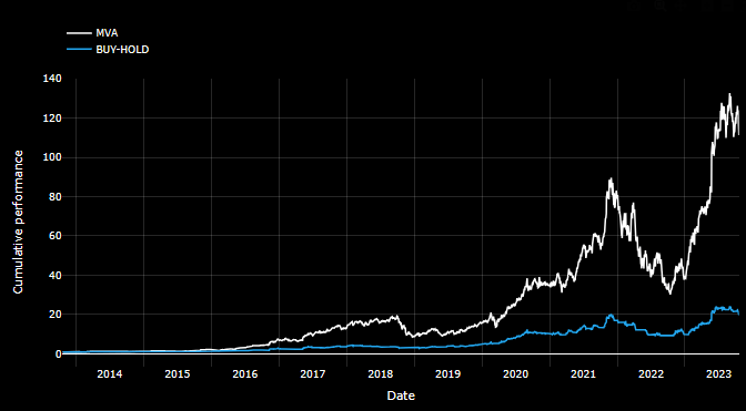
- Invoking Plotly to compare cumulative returns of MVA and Buy-Hold trading strategies
fig = go.Figure()
fig.add_trace(go.Scatter(x=ticker_history.index, y=ticker_history['cumulative_returns'], name='MVA',
                         line=dict(color='white', width=2)))
fig.add_trace(go.Scatter(x=ticker_history.index, y=ticker_history['cumulative_strategy_returns'], name='BUY-HOLD',
                         line=dict(color='#22a7f0', width=2)))
fig.update_layout(title=(''),
                  xaxis_title='Date',
                  yaxis_title='Cumulative performance',
                  font=dict(color='white'),
                  paper_bgcolor='black',
                  plot_bgcolor='black',
                  legend=dict(x=0, y=1.2, bgcolor='rgba(0,0,0,0)'),
                  yaxis=dict(gridcolor='rgba(255,255,255,0.2)'),
                  xaxis=dict(gridcolor='rgba(255,255,255,0.2)'))
fig.update_xaxes(showgrid=True, ticklabelmode="period")
fig.update_yaxes(showgrid=True)
fig.show()
- Calculating the maximum cumulative returns and the current drawdown of the strategy returns in relation to the maximum cumulative returns
#Calculate the maximum cumulative returns of the strategy so far
ticker_history['cumulative_strategy_max'] = ticker_history['cumulative_strategy_returns'].cummax()

#Calculate the current drawdown of the strategy returns in relation to the maximum cumulative returns
ticker_history['cumulative_strategy_drawdown'] = (ticker_history['cumulative_strategy_returns'] / ticker_history['cumulative_strategy_max']) - 1

#Print the current drawdown
print('The current drawdown of the strategy is:', ticker_history['cumulative_strategy_drawdown'][-1])
The current drawdown of the strategy is: -0.1868066793178107
- Calculating mean fast/slow 10-20 MVAs and strategy returns
#Define base slow and fast moving averages
fast_ma = 10
slow_ma = 20

#Calculate the moving averages for the strategy
ticker_history['fast_ma'] = ticker_history['Close'].rolling(window=fast_ma).mean()
ticker_history['slow_ma'] = ticker_history['Close'].rolling(window=slow_ma).mean()

#Create a column with buy and sell signals
ticker_history['signal'] = np.where(ticker_history['fast_ma'] > ticker_history['slow_ma'], 1.0, 0.0)

# Calculate daily ticker and strategy returns
ticker_history['returns'] = ticker_history['Close'].pct_change()
ticker_history['strategy_returns'] = ticker_history['signal'].shift(1) * ticker_history['returns']
Heatmap of MVA Returns
- Preparing data for heatmaps of returns
# Define two lists of fast and slow moving average values to be used as index and columns for a returns matrix
fast_ma_range = [5, 7, 9, 10, 20, 21, 30, 40, 50, 100]
slow_ma_range = [7, 9, 10, 20, 21, 30, 40, 50, 100, 200]

# Create a DataFrame with the index and columns as the fast and slow moving average values, respectively
# The DataFrame will be used to store returns data for different combinations of the moving averages
returns_matrix = pd.DataFrame(index=fast_ma_range, columns=slow_ma_range)
# Iterate through all combinations of fast and slow moving average values
for fast_ma in fast_ma_range:
    for slow_ma in slow_ma_range:

        # Calculate the fast and slow moving averages of the stock's closing price
        ticker_history['fast_ma'] = ticker_history['Close'].rolling(window=fast_ma).mean()
        ticker_history['slow_ma'] = ticker_history['Close'].rolling(window=slow_ma).mean()

        # Generate a signal to buy (1.0) or sell (0.0) based on the relative positions of the two moving averages
        ticker_history['signal'] = np.where(ticker_history['fast_ma'] > ticker_history['slow_ma'], 1.0, 0.0)

        # Calculate the daily returns of the stock and the strategy
        ticker_history['strategy_returns'] = ticker_history['signal'].shift(1) * ticker_history['returns']

        # Calculate the cumulative returns of the strategy
        cumulative_strategy_returns = (1 + ticker_history['strategy_returns']).cumprod()

        # Add the cumulative returns of the strategy to the returns matrix
        returns_matrix.loc[fast_ma, slow_ma] = cumulative_strategy_returns[-1]
# Make a copy of the returns_matrix and convert index and columns to string type
values = returns_matrix.copy()
values.index = values.index.astype(str)
values.columns = values.columns.astype(str)

# Convert values to float type
values = values.astype(float)

# Change the style of the plot and set the default color scheme
plt.style.use('dark_background')
sns.set_palette("bright")

# Create a heatmap with the provided values, including annotations, using the RdYlGn color map
sns.heatmap(values, annot=True, cmap='RdYlGn')

# Add labels to the axes
plt.xlabel('Slow Moving Average', fontsize=12, color='white')
plt.ylabel('Fast Moving Average', fontsize=12, color='white')

# Add a title to the plot
plt.title('Heatmap of Returns', fontsize=16, color='white')

# Increase the font size to 0.8 and change the color to white for all text elements
sns.set(font_scale=0.8, rc={'text.color':'white', 'axes.labelcolor':'white', 'xtick.color':'white', 'ytick.color':'white'})

# Change the background color of the plot to black
fig = plt.gcf()
fig.set_facecolor('#000000')

# Display the plot
plt.show()

Heatmap of MVA Drawdowns
- Preparing data for heatmaps of drawdowns
# Define two lists of fast and slow moving average values to be used as index and columns for a returns matrix
fast_ma_range = [5, 7, 9, 10, 20, 21, 30, 40, 50, 100]
slow_ma_range = [7, 9, 10, 20, 21, 30, 40, 50, 100, 200]

# Create a DataFrame with the index and columns as the fast and slow moving average values, respectively
# The DataFrame will be used to store returns data for different combinations of the moving averages
dd_matrix = pd.DataFrame(index=fast_ma_range, columns=slow_ma_range)
# Loop through different values for fast and slow moving averages
for fast_ma in fast_ma_range:
    for slow_ma in slow_ma_range:

        # Calculate the moving averages for the strategy
        ticker_history['fast_ma'] = ticker_history['Close'].rolling(window=fast_ma).mean()
        ticker_history['slow_ma'] = ticker_history['Close'].rolling(window=slow_ma).mean()

        # Create a binary signal column for buy/sell signals
        ticker_history['signal'] = np.where(ticker_history['fast_ma'] > ticker_history['slow_ma'], 1.0, 0.0)

        # Calculate daily returns for the ticker and the strategy
        ticker_history['strategy_returns'] = ticker_history['signal'].shift(1) * ticker_history['returns']

        # Calculate cumulative returns for the strategy
        ticker_history['cumulative_strategy_returns'] = (1 + ticker_history['strategy_returns']).cumprod()

        # Calculate maximum cumulative returns for the strategy
        ticker_history['cumulative_strategy_max'] = ticker_history['cumulative_strategy_returns'].cummax()

        # Calculate the drawdown for the strategy
        ticker_history['cumulative_strategy_drawdown'] = (ticker_history['cumulative_strategy_returns'] / ticker_history['cumulative_strategy_max']) - 1

        # Add drawdown to the matrix of drawdowns
        dd_matrix.loc[fast_ma, slow_ma] = ticker_history['cumulative_strategy_drawdown'][-1]
# Make a copy of the drawdown matrix and convert the index and columns to string type
values_dd = dd_matrix.copy()
values_dd.index = values_dd.index.astype(str)
values_dd.columns = values_dd.columns.astype(str)

# Convert values to float type
values_dd = values_dd.astype(float)

# Change the style of the plot and set the default color scheme
plt.style.use('dark_background')
sns.set_palette("bright")

# Create a heatmap with the provided values, including annotations, using the RdYlGn color map
sns.heatmap(values_dd, annot=True, cmap='RdYlGn')

# Add labels to the axes
plt.xlabel('Slow Moving Average', fontsize=12, color='white')
plt.ylabel('Fast Moving Average', fontsize=12, color='white')

# Add a title to the plot
plt.title('Heatmap of Drawdowns', fontsize=16, color='white')

# Increase the font size to 0.8 and change the color to white for all text elements
sns.set(font_scale=0.8, rc={'text.color':'white', 'axes.labelcolor':'white', 'xtick.color':'white', 'ytick.color':'white'})

# Change the background color of the plot to black
fig = plt.gcf()
fig.set_facecolor('#000000')

# Display the plot
plt.show()

Predicted RNN Trading Strategy Returns
- Downloading 15-min NVDA data from yfinance
import numpy as np
import pandas as pd
import yfinance as yf
import matplotlib.pyplot as plt
from sklearn.preprocessing import MinMaxScaler
from keras.models import Sequential
from keras.layers import Dense, SimpleRNN, Dropout
from keras.optimizers import Adam

# Download 15-minute NVDA data from yfinance
nvd = yf.Ticker('NVDA')
data = nvd.history(interval='15m', start='2023-10-03', end='2023-10-17')

# Reset the index to make 'Date' a regular column
data = data.reset_index()
data.tail()

- Implementing the RNN price prediction model
scaler = MinMaxScaler(feature_range=(0, 1))
scaled_data = scaler.fit_transform(data['Close'].values.reshape(-1, 1))

# Create training and testing datasets
def create_dataset(scaled_data, lookback=160):
    X, y = [], []
    for i in range(lookback, len(scaled_data)):
        X.append(scaled_data[i - lookback:i, 0])
        y.append(scaled_data[i, 0])
    return np.array(X), np.array(y)

lookback = 160
train_ratio = 0.95
train_size = int(len(scaled_data) * train_ratio)

train_data = scaled_data[:train_size]
test_data = scaled_data[train_size - lookback:]

X_train, y_train = create_dataset(train_data, lookback)
X_test, y_test = create_dataset(test_data, lookback)

X_train = np.reshape(X_train, (X_train.shape[0], X_train.shape[1], 1))
X_test = np.reshape(X_test, (X_test.shape[0], X_test.shape[1], 1))

# Build the RNN model
model = Sequential()
model.add(SimpleRNN(50, return_sequences=True, input_shape=(X_train.shape[1], 1)))
model.add(Dropout(0.2))
model.add(SimpleRNN(50, return_sequences=True))
model.add(Dropout(0.2))
model.add(SimpleRNN(50))
model.add(Dropout(0.2))
model.add(Dense(1))

model.compile(optimizer=Adam(lr=0.001), loss='mean_squared_error')

# Train the model
model.fit(X_train, y_train, epochs=100, batch_size=64)

# Make predictions
predicted_prices = model.predict(X_test)
predicted_prices = scaler.inverse_transform(predicted_prices)

# Evaluate the model
rmse = np.sqrt(np.mean((predicted_prices - y_test)**2))
print('Root Mean Squared Error:', rmse)

# Plotting the predicted against the actual
num_test_points = len(X_test)
test_datetime_values = data.iloc[-num_test_points:, 0]

# Inverse transform the actual prices (y_test)
actual_prices = scaler.inverse_transform(y_test.reshape(-1, 1))

# Plot actual and predicted stock prices
fig=plt.figure(figsize=(12, 5))
import matplotlib as mpl
mpl.rcParams['text.color'] = 'blue'
mpl.rcParams.update({'font.size': 22})
mpl.rcParams['xtick.labelcolor'] = 'blue'
mpl.rcParams['xtick.color'] = 'blue'
mpl.rcParams['ytick.labelcolor'] = 'blue'
mpl.rcParams['ytick.color'] = 'blue'

plt.plot(test_datetime_values, actual_prices, label='Actual Prices',lw=4)
plt.plot(test_datetime_values, predicted_prices, label='Predicted Prices',lw=4)

font1 = {'family':'sans-serif','color':'blue','size':20}
plt.xlabel('Datetime',fontdict = font1)
plt.ylabel('Stock Prices',fontdict = font1)
plt.title('NVDA Stock Price Prediction')
plt.rcParams.update({'text.color': "blue",
                     'axes.labelcolor': "blue"})
plt.legend()

SMALL_SIZE = 16
MEDIUM_SIZE = 16
BIGGER_SIZE = 16

plt.rc('font', size=SMALL_SIZE)          # controls default text sizes
plt.rc('axes', titlesize=SMALL_SIZE)     # fontsize of the axes title
plt.rc('axes', labelsize=MEDIUM_SIZE)    # fontsize of the x and y labels
plt.rc('xtick', labelsize=SMALL_SIZE)    # fontsize of the tick labels
plt.rc('ytick', labelsize=SMALL_SIZE)    # fontsize of the tick labels
plt.rc('legend', fontsize=SMALL_SIZE)    # legend fontsize
plt.rc('figure', titlesize=BIGGER_SIZE)  # fontsize of the figure
plt.grid(c='black')
plt.show()

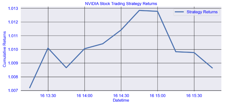
- Plotting cumulative RNN strategy returns
# Calculate the percentage change in predicted prices
predicted_pct_change = np.diff(predicted_prices.reshape(-1)) / predicted_prices[:-1].reshape(-1)

# Get the actual prices corresponding to the predicted_prices in the test set
actual_prices_test = actual_prices[-len(predicted_prices) + 1:]

# Calculate the percentage change in actual prices
actual_pct_change = np.diff(actual_prices_test.reshape(-1)) / actual_prices_test[:-1].reshape(-1)

# Truncate the longer array if the lengths are not equal
if len(predicted_pct_change) != len(actual_pct_change):
    min_len = min(len(predicted_pct_change), len(actual_pct_change))
    predicted_pct_change = predicted_pct_change[:min_len]
    actual_pct_change = actual_pct_change[:min_len]

# Create a trading strategy based on the predicted percentage change
strategy_returns = np.where(predicted_pct_change > 0, 1, -1) * actual_pct_change

# Calculate the cumulative returns
cumulative_returns = (1 + strategy_returns).cumprod()

# Plot the cumulative returns
import matplotlib as mpl
mpl.rcParams['text.color'] = 'blue'
plt.figure(figsize=(14, 6))
plt.plot(data['Datetime'].iloc[-len(cumulative_returns):], cumulative_returns, label='Strategy Returns',lw=4)
plt.xlabel('Datetime')
plt.ylabel('Cumulative Returns')
plt.title('NVIDIA Stock Trading Strategy Returns')
plt.legend()
plt.grid(c='black')
plt.show()
- Predicting RNN mean reversion strategy returns
import yfinance as yf
import numpy as np
import pandas as pd
from sklearn.preprocessing import MinMaxScaler
from tensorflow.keras.models import Sequential
from tensorflow.keras.layers import LSTM, Dense, Dropout
from tensorflow.keras.layers import SimpleRNN

# Download 15-minute NVIDIA data from yfinance
tesla = yf.download('NVDA', start='2023-10-03', end='2023-10-17', interval='15m')

# Reset the index
tesla.reset_index(inplace=True)

# Preprocess data
data = tesla[['Close']]
scaler = MinMaxScaler(feature_range=(0, 1))
scaled_data = scaler.fit_transform(data)


# Create a Function that generates 'good' data for the process
def create_dataset(data, lookback):
    features, targets = [], []
    for i in range(lookback, len(data)):
        features.append(data[i-lookback:i])
        targets.append(data[i, 0])
    return np.array(features), np.array(targets)

lookback = 60
mean_reversion_features, mean_reversion_targets = create_dataset(scaled_data, lookback)

# Split data into train and test
train_size = int(len(mean_reversion_features) * 0.8)

X_train_mean_reversion, y_train_mean_reversion = mean_reversion_features[:train_size], mean_reversion_targets[:train_size]
X_test_mean_reversion, y_test_mean_reversion = mean_reversion_features[train_size:], mean_reversion_targets[train_size:]

X_train_mean_reversion = X_train_mean_reversion.reshape((X_train_mean_reversion.shape[0], X_train_mean_reversion.shape[1], 1))
X_test_mean_reversion = X_test_mean_reversion.reshape((X_test_mean_reversion.shape[0], X_test_mean_reversion.shape[1], 1))

def create_rnn_model(lookback):
    model = Sequential()
    model.add(SimpleRNN(units=50, return_sequences=True, input_shape=(lookback, 1)))
    model.add(SimpleRNN(units=50, return_sequences=False))
    model.add(Dense(units=25))
    model.add(Dense(units=1))
    model.compile(optimizer='adam', loss='mean_squared_error')
    return model

mean_reversion_rnn = create_rnn_model(lookback)

# Train the model
mean_reversion_rnn.fit(X_train_mean_reversion, y_train_mean_reversion, epochs=5, batch_size=32)

# Generate predictions
y_test_mean_reversion = mean_reversion_rnn.predict(X_test_mean_reversion)

# Calculate the z-score of predicted mean reversion values
z_scores = (y_test_mean_reversion - y_test_mean_reversion.mean()) / y_test_mean_reversion.std()

# Define z-score threshold for buy and sell signals
z_threshold = 1

# Generate trading signals
mean_reversion_signals = np.where(z_scores > z_threshold, -1, np.where(z_scores < -z_threshold, 1, 0))

last_train_index = tesla.index[train_size + lookback - 1]

returns = np.diff(tesla.loc[last_train_index + 1:, 'Close'].values) * mean_reversion_signals.flatten()[:-1]

# Calculate cumulative returns
cumulative_returns = np.cumsum(returns)

# Plot cumulative returns
plt.figure(figsize=(14, 6))
plt.plot(tesla.loc[last_train_index + 2:, 'Datetime'].values, cumulative_returns, label='Mean Reversion Strategy Returns',lw=4)
plt.xlabel('Datetime')
plt.ylabel('Cumulative Returns')
plt.legend()
plt.grid(c='black')
plt.show()

Summary
- The 10Y MVA optimized strategy 40-200 yields cumulative return of 130% and max drawdown of -16%. The choice of different MVAs can affect the results of the MVA strategy. In addition, commissions should be added to the analysis, as well as the effect of slippage.
- The 14-day RNN mean reversion strategy cumulative return is 3%. There are significant plateau periods in both the actual data (when the markets are closed) and the model returns for the same reason.
Explore More


One-Time
Monthly
Yearly
Make a one-time donation
Make a monthly donation
Make a yearly donation
Choose an amount
€5.00
€15.00
€100.00
€5.00
€15.00
€100.00
€5.00
€15.00
€100.00
Or enter a custom amount
€
Your contribution is appreciated.
Your contribution is appreciated.
Your contribution is appreciated.
DonateDonate monthlyDonate yearly
Leave a comment