
- The objective of this post is to predict the STD-related volatility of the NVIDIA stock by comparing the following two TSA models in Python: (1) the Generalized Autoregressive Conditional Heteroscedasticity (GARCH) statistical forecast model and (2) the Extreme Gradient Boosting (XGBoost) supervised Machine Learning (ML) model.
- The GARCH model describes the time-varying variance of financial time series data. It is commonly used to model volatility of financial returns, and can be used to make predictions of volatility.
- XGBoost regression is the most famous ML algorithm to handle different types of structured data. Using trading technical indicators (TTIs) as features, one can employ XGBoost to predict future stock trends and prices.
Table of Contents
- Why NVIDIA
- Basic Imports
- Input NVIDIA Stock Data
- NVIDIA Stock Volatility Analysis
- GARCH Volatility Prediction
- XGBoost Volatility Prediction
- GARCH vs XGBoost Comparisons
- Summary
- Explore More
Why NVIDIA
NVIDIA reported revenue for the Q2 ended July 30, 2023, of $13.51 billion, up 101% from a year ago and up 88% from the previous quarter. GAAP earnings per diluted share for the quarter were $2.48, up 854% from a year ago and up 202% from the previous quarter. Non-GAAP earnings per diluted share were $2.70, up 429% from a year ago and up 148% from the previous quarter.

- NVIDIA stock is expected to more than double within the next year (The Motley Fool)
- Zacks: Zacks’ proprietary data indicates that NVIDIA Corporation is currently rated as a Zacks Rank 1 and we are expecting an above average return from the NVDA shares relative to the market in the next few months. In addition, NVIDIA Corporation has a VGM Score of C (this is a weighted average of the individual Style Scores which allow you to focus on the stocks that best fit your personal trading style). Recent price changes and earnings estimate revisions indicate this would be a good stock for momentum investors with a Momentum Score of A.
- Stock Analysis: The average analyst rating for NVIDIA stock from 40 stock analysts is “Strong Buy”.

- Riding high on the AI wave, chip giant Nvidia (NVDA), emerged as a winner with its stock surging to record highs, making it the first chip maker to hit $1tn market capitalisation. Nvidia is the powerhouse behind semiconductors that power AI programs like ChatGPT, and saw an uptick in demand and revenues in the latest quarter.
- Trading View NVIDIA Charts & Key Stats:
Market capitalization 1.05TUSD
Dividends yield (FY) 0.04%
Price to earnings Ratio (TTM) 111.35
Basic EPS (TTM) 4.18USD
Net income 4.368BUSD
Revenue 26.974BUSD
Shares float 2.37B
Basic Imports
Let’s set the working directory YOURPATH and import key libraries
import os
os.chdir('YOURPATH')    # Set working directory
os. getcwd()
import math
import datetime
import warnings
import numpy as np
import pandas as pd
import plotly.express as px
import plotly.figure_factory as ff
import matplotlib.pyplot as plt
import seaborn as sns
import xgboost as xgb
from arch import arch_model
from statsmodels.graphics.tsaplots import plot_acf, plot_pacf
from ipywidgets import HBox, VBox
from tabulate import tabulate
from sklearn.metrics import mean_absolute_percentage_error
from sklearn.metrics import mean_squared_error
from xgboost import plot_importance, plot_tree
#Matplotlib style
plt.style.use('fivethirtyeight')
#Ignoring some warnings
warnings.filterwarnings('ignore')
Input NVIDIA Stock Data
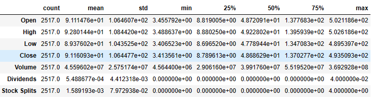
Let’s download the 10Y stock data and perform the preliminary data analysis
import numpy as np
import pandas as pd
import yfinance as yf

import matplotlib.pyplot as plt
import plotly.graph_objs as go
import seaborn as sns
#Download ticker price data from yfinance
tick = 'NVDA'
ticker = yf.Ticker(tick)
ticker_history = ticker.history(period='10y')
ticker_history.tail()

ticker_history.shape
(2517, 7)
ticker_history.info()
<class 'pandas.core.frame.DataFrame'>
DatetimeIndex: 2517 entries, 2013-10-18 00:00:00-04:00 to 2023-10-18 00:00:00-04:00
Data columns (total 7 columns):
 #   Column        Non-Null Count  Dtype
---  ------        --------------  -----
 0   Open          2517 non-null   float64
 1   High          2517 non-null   float64
 2   Low           2517 non-null   float64
 3   Close         2517 non-null   float64
 4   Volume        2517 non-null   int64
 5   Dividends     2517 non-null   float64
 6   Stock Splits  2517 non-null   float64
dtypes: float64(6), int64(1)
memory usage: 157.3 KB
ticker_history.describe().T
NVIDIA Stock Volatility Analysis
#Calculate the percentage change by day
returns_nvd = 100 * ticker_history.Close.pct_change().dropna()
#Drop 0 results, there is a error in the dataset and for 74 days,the stock market was close, so the return is 0
returns_nvd = returns_nvd.drop(returns_nvd[returns_nvd == 0].index)
#Display the 3 first rows of the Serie
returns_nvd.tail()
Date
2023-10-12 00:00:00-04:00    0.296974
2023-10-13 00:00:00-04:00   -3.161152
2023-10-16 00:00:00-04:00    1.394608
2023-10-17 00:00:00-04:00   -4.679468
2023-10-18 00:00:00-04:00   -3.760917
Name: Close, dtype: float64
#Average of return column
returns_nvd.mean()
0.23128969312944928
#Using the raw close prices to plot the evolution of the stock
close_prices = pd.DataFrame(ticker_history["Close"])
#By dividing each close price by the first price in our dataset we calculate the accumulated return for each day
cum_rets = close_prices / close_prices.iloc[0,:]
#Using the plotly.express module we can plot our newly created cum_rets
fig = px.line(cum_rets.iloc[:,:], width=1000, height=500)
#Adding Title
fig.update_layout(title_text='10Y Cumulative Return of NVDA Stock')
#This will print the graph
fig.show()

#The daily volatility is the std of the returns
daily_volatility = returns_nvd.std()
#The monthly volatility is the result of multiplying the daily vol * square root of 21, this is because there are 21 trading days in a month
monthly_volatility = math.sqrt(21) * daily_volatility
#The annual volatility is the result of multiplying the daily vol * square root of 252, this is because there are 252 trading days in a year
annual_volatility = math.sqrt(252) * daily_volatility
#Using tabulate package we can print a nice table
print(tabulate([['nvd',daily_volatility,monthly_volatility,annual_volatility]],headers = ['Daily Volatility %', 'Monthly Volatility %', 'Annual Volatility %'],tablefmt = 'fancy_grid',stralign='center',numalign='center',floatfmt=".2f"))
╒═════╤══════════════════════╤════════════════════════╤═══════════════════════╕
│     │  Daily Volatility %  │  Monthly Volatility %  │  Annual Volatility %  │
╞═════╪══════════════════════╪════════════════════════╪═══════════════════════╡
│ nvd │         2.92         │         13.39          │         46.38         │
╘═════╧══════════════════════╧════════════════════════╧═══════════════════════╛
#We can plot the daily retuns of nvda using a line graph .plot from pandas
returns_nvd.plot(figsize =(16,5), title = 'NVDA Daily Returns');

#We create a distribution plot using plotly.figure_factory, we reshape the data to have them in a vector
return_dist_plot  = ff.create_distplot([returns_nvd.values.reshape(-1)], group_labels = [' '])
#We specify the plot layout
return_dist_plot.update_layout(showlegend=False, title_text='Distribution of Daily NVDA Returns', width=1000, height=500)
#Printing the plot
return_dist_plot.show()

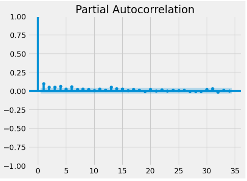
#This code uses the pacf() function from the tsa.stattools module of the statsmodels library (sm) to compute the autocorrelation function.
plot_pacf(returns_nvd**2,method="yw")
#Print the visualization
plt.show()
GARCH Volatility Prediction
#Define a GARCH model (4,4) that uses a ged distribution
model = arch_model(returns_nvd,dist="ged", vol = 'GARCH', p=4, q=4)
#Fit the model
model_fit = model.fit(disp='off')
#Summary of the model
model_fit.summary()
Model Fit Output:

Define the full series as the previosly defined model
full_serie_garch = arch_model(returns_nvd,dist="ged", vol = 'GARCH', p=4, q=4)
#Fitting the model for the full serie
model_fit_full_serie = full_serie_garch.fit(disp='off')
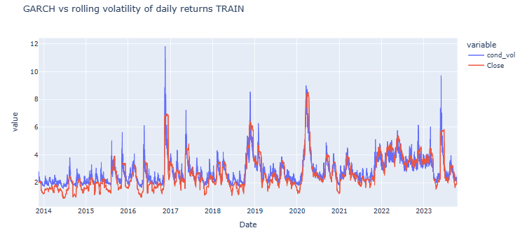
#We will plot against the rolling volatility
rolling_vol = abs(returns_nvd.rolling(window=22, min_periods=22).std().dropna())
#Concatenating the true values, and trained values in our model
garch_and_rolling_std = pd.concat([pd.DataFrame(model_fit_full_serie.conditional_volatility),rolling_vol.dropna()], axis=1).dropna()
#Plotting it
garch_and_rolling_std_plot = px.line(garch_and_rolling_std, title = 'GARCH vs rolling volatility of daily returns TRAIN', width=1000, height=500)
#Printing the plot
garch_and_rolling_std_plot.show()
#Using a numeric range of 251 to fill a list of predicted values, for each day we are fitting a new model with the same parameters, but adding the last day.
test_size = 251
rolling_predictions = []

for i in range(test_size):
    train = returns_nvd[:-(test_size-i)]
    model = arch_model(train,dist="ged", vol = 'GARCH', p=4, q=4)
    model_fit = model.fit(disp='off')
    pred = model_fit.forecast(horizon=1, reindex = False)
    rolling_predictions.append(np.sqrt(pred.variance.values[-1,:][0]))
#Transforming it to a series
rolling_predictions = pd.Series(rolling_predictions, index= returns_nvd.dropna().index[-test_size:])
#Setting plot parameters
plt.figure(figsize=(10,4))
#True data
true, = plt.plot((rolling_vol)[-test_size:])
#Predicted data
preds, = plt.plot(rolling_predictions)
#Plot of the data
plt.title('Volatility Prediction for the next 251 Trading Days - Rolling Forecast TEST with GARCH(4,4)', fontsize=20)
#Add legend
plt.legend(['True Volatility', 'Predicted Volatility'], fontsize=16)

XGBoost Volatility Prediction
Let’s prepare the data
nvd_stock_raw_data_for_ml = ticker_history.copy()
nvd_stock_raw_data_for_ml.reset_index(inplace=True)
#XGBoost
#We only need the date and close columns
returns_nvd_for_ml = nvd_stock_raw_data_for_ml[["Date","Close"]]
#We change the close column for the percentual change calculation
returns_nvd_for_ml["Close"] = 100 * returns_nvd_for_ml.Close.pct_change().dropna()
#Drop 0 returns
returns_nvd_for_ml  = returns_nvd_for_ml.drop(returns_nvd_for_ml[returns_nvd_for_ml["Close"] == 0].index)
#Drop N/A
returns_nvd_for_ml = returns_nvd_for_ml.dropna()
#As we will be comparing it to the rolling volatility of 22 days, we will transform our target to that
returns_nvd_for_ml["Close"] = abs(returns_nvd_for_ml["Close"].rolling(window=22, min_periods=22).std().dropna())
#Convert the date column to datetime format
returns_nvd_for_ml["Date"] = pd.to_datetime(returns_nvd_for_ml["Date"])
#Rename the dataframe
serie_for_xgboost = returns_nvd_for_ml
#Set the test size
test_size = 251
#Split train and test
train_ml = serie_for_xgboost[:-(test_size)].dropna()
test_ml = serie_for_xgboost[-(test_size):].dropna()
#Function for extracting features from date
def create_features(df, label=None):
    """
    Creates time series features from datetime index
    """
    df['dayofweek'] = df['Date'].dt.dayofweek
    df['quarter'] = df['Date'].dt.quarter
    df['month'] = df['Date'].dt.month
    df['year'] = df['Date'].dt.year
    df['dayofyear'] = df['Date'].dt.dayofyear
    df['dayofmonth'] = df['Date'].dt.day


    X = df[['dayofweek','quarter','month','year',
           'dayofyear','dayofmonth']]
    if label:
        y = df[label]
        return X, y
    return X
#Creating the features for the train and test sets
X_train, y_train = create_features(train_ml, label="Close")
X_test, y_test = create_features(test_ml, label="Close")
#Defining and fitting the model
reg = xgb.XGBRegressor(n_estimators=1000,early_stopping_rounds=50,)
reg.fit(X_train, y_train,
        eval_set=[(X_train, y_train), (X_test, y_test)],
       verbose=False)
XGBRegressor
XGBRegressor(base_score=0.5, booster='gbtree', callbacks=None,
             colsample_bylevel=1, colsample_bynode=1, colsample_bytree=1,
             early_stopping_rounds=50, enable_categorical=False,
             eval_metric=None, feature_types=None, gamma=0, gpu_id=-1,
             grow_policy='depthwise', importance_type=None,
             interaction_constraints='', learning_rate=0.300000012, max_bin=256,
             max_cat_threshold=64, max_cat_to_onehot=4, max_delta_step=0,
             max_depth=6, max_leaves=0, min_child_weight=1, missing=nan,
             monotone_constraints='()', n_estimators=1000, n_jobs=0,
             num_parallel_tree=1, predictor='auto', random_state=0, ...)
#Plot of feature importance
_ = plot_importance(reg, height=0.9)

#Predicting with our model for both the train and test data
train_ml["Predictions"] = reg.predict(X_train)
test_ml['Prediction'] = reg.predict(X_test)
#Creating the dataframe with both real and predicted vol
XGBoost_and_rolling = pd.concat([pd.DataFrame(list(train_ml["Predictions"]),list(train_ml["Close"]))], axis=1).dropna().reset_index()
#Renaming columns
XGBoost_and_rolling.rename(columns={"index":"Real_Volatility",0:"Predicted Volatility"}, inplace=True)
XGBoost_and_rolling.head(10)
Real_Volatility	Predicted Volatility
0	2.004440	1.991486
1	2.025624	1.995968
2	2.033402	1.981669
3	2.011338	2.058352
4	2.059768	1.995043
5	2.051825	2.018471
6	2.050722	2.058352
7	2.058269	1.981669
8	2.064700	2.006868
9	2.063672	2.006868
#Plotting the predictions of the training data
XGBoost_and_rolling = pd.concat([pd.DataFrame(list(train_ml["Predictions"]),list(train_ml["Close"]))], axis=1).dropna().reset_index()
XGBoost_and_rolling.rename(columns={"index":"Real_Volatility",0:"Predicted Volatility"}, inplace=True)
XGBoost_and_rolling = px.line(XGBoost_and_rolling, title = 'XGBOOST vs Rolling Volatility of Daily Returns TRAIN', width=1000, height=500)
XGBoost_and_rolling.show()

#Plotting the predictions for the test data
plt.figure(figsize=(10,4))
true, = plt.plot(test_ml["Close"])
preds, = plt.plot(test_ml['Prediction'])
plt.title('Volatility Prediction for the next 251 Trading Days - Rolling Forecast TEST with XGBOOST', fontsize=20)
plt.legend(['True Returns', 'Predicted Volatility'], fontsize=16)

GARCH vs XGBoost Comparisons
Let’s compare GARCH vs XGBoost results:
- GARCH model
RMSE_Serie = mean_squared_error(garch_and_rolling_std["Close"],garch_and_rolling_std["cond_vol"],squared=False)
MAPE_Serie = mean_absolute_percentage_error(garch_and_rolling_std["Close"], garch_and_rolling_std["cond_vol"])
print(f"The RMSE of our GARCH model in the full series data is {round(RMSE_Serie,4)}")
print(f"The MAPE of our GARCH model in the full series data is {round(MAPE_Series*100,2)}%")
The RMSE of our GARCH model in the full series data is 0.5975
The MAPE of our GARCH model in the full series data is 19.5%
true_vol = rolling_vol[-test_size:]
pred_vol = rolling_predictions
RMSE = mean_squared_error(true_vol, pred_vol,squared=False)
MAPE = mean_absolute_percentage_error(true_vol, pred_vol)
print(f"The RMSE of our GARCH model in the predicted data is {round(RMSE,4)}")
print(f"The MAPE of our GARCH model in the predicted data is {round(MAPE*100,2)}%")
The RMSE of our GARCH model in the predicted data is 0.7267
The MAPE of our GARCH model in the predicted data is 14.72%
- XGBOOST model
RMSE_Serie_XG = mean_squared_error(train_ml["Close"],train_ml["Predictions"],squared=False)
MAPE_Serie_XG = mean_absolute_percentage_error(train_ml["Close"], train_ml["Predictions"])
print(f"The RMSE of our XGBOOST model in the full series data is {round(RMSE_Serie_XG,4)}")
print(f"The MAPE of our XGBOOST model in the full series data is {round(MAPE_Serie_XG*100,2)}%")
The RMSE of our XGBOOST model in the full series data is 0.1482
The MAPE of our XGBOOST model in the full series data is 3.72%
true_vol = test_ml['Prediction']
pred_vol = test_ml["Close"]
RMSE_XG = mean_squared_error(true_vol, pred_vol,squared=False)
MAPE_XG = mean_absolute_percentage_error(true_vol, pred_vol)
print(f"The RMSE of our XGBOOST model in the predicted data is {round(RMSE_XG,4)}")
print(f"The MAPE of our XGBOOST model in the predicted data is {round(MAPE_XG*100,2)}%")
The RMSE of our XGBOOST model in the predicted data is 0.3728
The MAPE of our XGBOOST model in the predicted data is 5.76%
- GARCH vs XGBOOST
print(tabulate([['MAPE',round(MAPE_Serie*100,2),round(MAPE_Serie_XG*100,2),round(MAPE*100,2),round(MAPE_XG*100,2)]],headers = ['GARCH TRAIN %', 'XGBOOST TRAIN %', 'GARCH PREDICTIONS %','XGBOOST PREDICTIONS %'],tablefmt = 'fancy_grid',stralign='center',numalign='center',floatfmt=".2f"))
╒══════╤═════════════════╤═══════════════════╤═══════════════════════╤═════════════════════════╕
│      │  GARCH TRAIN %  │  XGBOOST TRAIN %  │  GARCH PREDICTIONS %  │  XGBOOST PREDICTIONS %  │
╞══════╪═════════════════╪═══════════════════╪═══════════════════════╪═════════════════════════╡
│ MAPE │      19.22      │       2.01        │         14.67         │          7.19           │
╘══════╧═════════════════╧═══════════════════╧═══════════════════════╧═════════════════════════╛
Summary
- The GARCH and XGBoost models have been used to predict the NVDA volatility.
- GARCH is a widely-used statistical model for forecasting the variance of financial time series.
- A comparison of GARCH and XGBoost in terms of MAPE and RMSE has been accomplished.
- Results show that the XGBoost model is able to accurately predict the rolling monthly volatility of NVDA and outperforms the GARCH model in out-of-sample forecasting.
- This project supports previous studies in that it demonstrates the usefulness of supervised ML in stock volatility forecasting and highlights the importance of considering the time-varying nature of volatility in quantitative financial analysis.
Explore More
- Predicting Volatility: GARCH vs XGBoost
- IQR-Based Log Price Volatility Ranking of Top 19 Blue Chips
- Multiple-Criteria Technical Analysis of Blue Chips in Python
- Blue-Chip Stock Portfolios for Quant Traders
- Are Blue Chips Perfect for This Bear Market?


Make a one-time donation
Make a monthly donation
Make a yearly donation
Choose an amount
Or enter a custom amount
Your contribution is appreciated.
Your contribution is appreciated.
Your contribution is appreciated.
DonateDonate monthlyDonate yearly
Leave a comment