
- Today the focus is on risk assessment of top blue chips (NVDA, ORCL, AMD, AAPL, INTC, AMZN, GE, XOM, TSLA, MSFT, WMT, PG, KO, JNJ, BAC, NKE, HON, GS, and ^GSPC) using the IQR-based real-time volatility ranking algorithm and the corresponding Python functions.
- The objective is to determine market regimes using standard deviation (STD) of log-domain stock prices. It allows us to assess how values in a dataset are distributed around the mean.
- Let’s set the working directory YOURPATH
import os
os.chdir('YOURPATH')    # Set working directory
os. getcwd()
- Consider the class Levels
import pandas as pd
import numpy as np
import matplotlib.pyplot as plt
import matplotlib.patches as mpatches

class Levels:
    def run(self):
        df = self.read_file()
        df = self.calc_std_dev_levels(df)
        self.plot_levels(df)

    def read_file(self):
        filename = 'data.csv'
        df = pd.read_csv(filename, names=['receive_timestamp', 'price'])
        df['receive_timestamp'] = pd.to_datetime(df['receive_timestamp'])
        df.set_index('receive_timestamp', inplace=True)
        return df

    def calc_std_dev_levels(self, df):
        #log price
        df['price'] = df['price'].apply(np.log)
        #price difference
        df['price_diff'] = df['price'].diff()
        #std dev
        df['std_dev'] = df['price_diff'].rolling(window=100).std()
        #use rolling mean to find 'zones' of volatility
        df['std_dev_ma'] = df['std_dev'].rolling(3000).mean()
        #thresholds between levels
        std_dev_ma_threshold_1 = df['std_dev_ma'].quantile(0.2)
        std_dev_ma_threshold_2 = df['std_dev_ma'].quantile(0.4)
        std_dev_ma_threshold_3 = df['std_dev_ma'].quantile(0.6)
        std_dev_ma_threshold_4 = df['std_dev_ma'].quantile(0.8)
        # Initialize 'signal' column with zeros
        df['levels'] = 0
        #assign levels based on average std dev
        df.loc[(df['std_dev_ma'] > std_dev_ma_threshold_1), 'levels'] = 1
        df.loc[(df['std_dev_ma'] > std_dev_ma_threshold_2), 'levels'] = 2
        df.loc[(df['std_dev_ma'] > std_dev_ma_threshold_3), 'levels'] = 3
        df.loc[(df['std_dev_ma'] > std_dev_ma_threshold_4), 'levels'] = 4
        return df

    def plot_levels(self, df):
        fig, ax = plt.subplots()
        colors = {
            0:'grey',
            1:'green',
            2: 'blue',
            3: 'red',
            4: 'black'
        }
        scatter = ax.scatter(
            np.reshape(df.index, -1),
            np.reshape(df['price'], -1),
            c=np.reshape(df['levels'].apply(lambda x: colors[x]), -1),
            s=10,
            linewidths=1
        )
        # Create proxy artists for legend
        legend_labels = [f'Level {level}' for level in colors.keys()]
        legend_handles = [mpatches.Patch(color=colors[level], label=label) for level, label in enumerate(legend_labels)]

        # Create a legend
        ax.legend(handles=legend_handles, title='Levels')

        plt.title('std dev levels')
        plt.xlabel('Date')
        plt.ylabel('Price')
        plt.grid(True)
        plt.show()
- Let’s test this class using the high-volatility segment data.csv
if __name__ == '__main__':
    v = Levels()
    v.run()
- Let’s take a closer look at the output

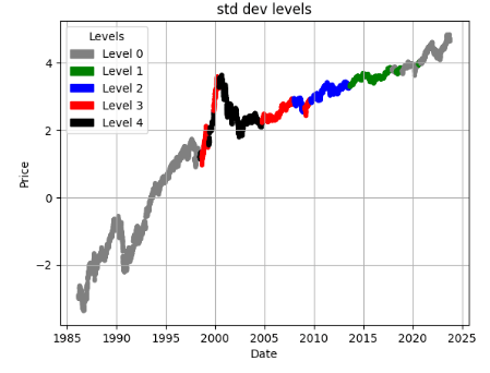
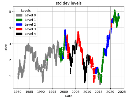
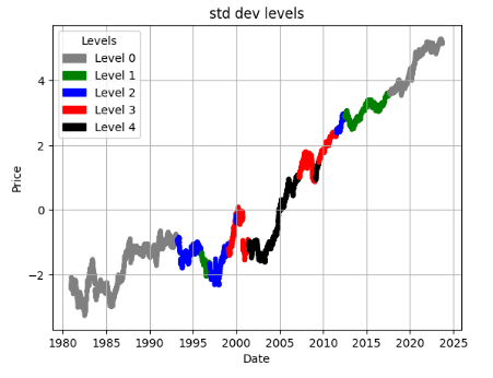
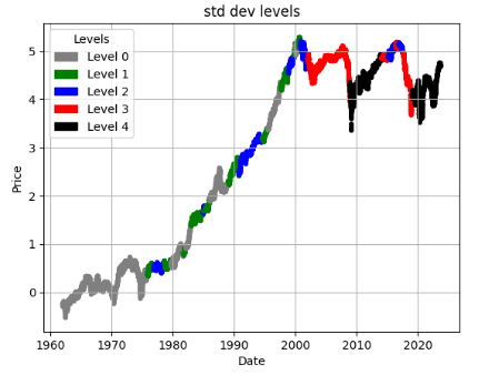
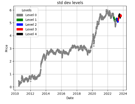
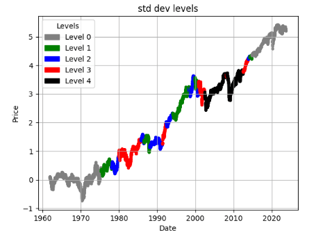
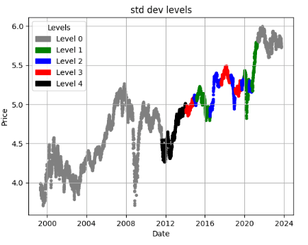
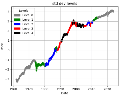
- Clearly, we can create a price chart and mark our levels. The faster the price changes, the higher the volatility and STD. Level 0 will correspond to the lowest volatility, with each subsequent group representing higher volatility. Gray and green zones represent low volatility, while red and black indicate the most volatile segments.
- Let’s replace the above class with the following two functions
# Importing Libraries

# Data Handling
import pandas as pd
import numpy as np

# Financial Data Analysis
import yfinance as yf

# Data Visualization
import plotly.express as px
import plotly.graph_objs as go
import plotly.subplots as sp
from plotly.subplots import make_subplots
import plotly.figure_factory as ff
import plotly.io as pio
from IPython.display import display
from plotly.offline import init_notebook_mode

# Statistics & Mathematics
import scipy.stats as stats
import statsmodels as sm
from scipy.stats import shapiro, skew
import math

# Hiding warnings
import warnings
warnings.filterwarnings("ignore")
def load_and_preprocess(ticker):
    '''
    This function takes in a ticker symbol, which is used to
    retrieve historical data from Yahoo Finance.
    The attributes 'Returns', and the Adjusted Low, High, and Open
    are created.
    NaNs are filled with 0s
    '''

    df = yf.download(ticker)
    df['Returns'] = df['Adj Close'].pct_change(1)
    df['Adj Low'] = df['Low'] - (df['Close'] - df['Adj Close'])
    df['Adj High'] = df['High'] - (df['Close'] - df['Adj Close'])
    df['Adj Open'] = df['Open'] - (df['Close'] - df['Adj Close'])
    df = df.fillna(0)
    return df
import matplotlib.pyplot as plt
import matplotlib.patches as mpatches
def plot_levels(df):
        #log price
        df['price'] = df['Adj Close'].apply(np.log)
        #price difference
        df['price_diff'] = df['price'].diff()


         #std dev
        df['std_dev'] = df['price_diff'].rolling(window=100).std()
        #use rolling mean to find 'zones' of volatility
        df['std_dev_ma'] = df['std_dev'].rolling(3000).mean()
        #thresholds between levels
        std_dev_ma_threshold_1 = df['std_dev_ma'].quantile(0.2)
        std_dev_ma_threshold_2 = df['std_dev_ma'].quantile(0.4)
        std_dev_ma_threshold_3 = df['std_dev_ma'].quantile(0.6)
        std_dev_ma_threshold_4 = df['std_dev_ma'].quantile(0.8)
        # Initialize 'signal' column with zeros
        df['levels'] = 0
        #assign levels based on average std dev
        df.loc[(df['std_dev_ma'] > std_dev_ma_threshold_1), 'levels'] = 1
        df.loc[(df['std_dev_ma'] > std_dev_ma_threshold_2), 'levels'] = 2
        df.loc[(df['std_dev_ma'] > std_dev_ma_threshold_3), 'levels'] = 3
        df.loc[(df['std_dev_ma'] > std_dev_ma_threshold_4), 'levels'] = 4

        fig, ax = plt.subplots()
        colors = {
            0:'grey',
            1:'green',
            2: 'blue',
            3: 'red',
            4: 'black'
        }
        scatter = ax.scatter(
            np.reshape(df.index, -1),
            np.reshape(df['price'], -1),
            c=np.reshape(df['levels'].apply(lambda x: colors[x]), -1),
            s=10,
            linewidths=1
        )
        # Create proxy artists for legend
        legend_labels = [f'Level {level}' for level in colors.keys()]
        legend_handles = [mpatches.Patch(color=colors[level], label=label) for level, label in enumerate(legend_labels)]

        # Create a legend
        ax.legend(handles=legend_handles, title='Levels')

        plt.title('std dev levels')
        plt.xlabel('Date')
        plt.ylabel('Price')
        plt.grid(True)
        plt.show()
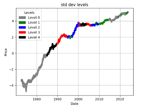
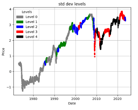
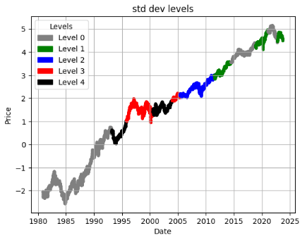
- Now, we can examine price := (log Adj Close price) charts of stocks and mark their STD levels as follows
ticker = 'NVDA'

df = load_and_preprocess(ticker)
plot_levels(df)

ticker = 'ORCL'

df = load_and_preprocess(ticker)
plot_levels(df)
ticker = 'AMD'

df = load_and_preprocess(ticker)
plot_levels(df)
ticker = 'XOM'

df = load_and_preprocess(ticker)
plot_levels(df)

ticker = 'AAPL'

df = load_and_preprocess(ticker)
plot_levels(df)
ticker = 'INTC'

df = load_and_preprocess(ticker)
plot_levels(df)

ticker = 'AMZN'

df = load_and_preprocess(ticker) # Loading and Transforming Dataframe
plot_levels(df)

ticker = 'GE'

df = load_and_preprocess(ticker) # Loading and Transforming Dataframe
plot_levels(df)
ticker = 'TSLA'

df = load_and_preprocess(ticker)
plot_levels(df)
ticker = 'MSFT'

df = load_and_preprocess(ticker)
plot_levels(df)

ticker = 'WMT'

df = load_and_preprocess(ticker)
plot_levels(df)
ticker = 'PG'

df = load_and_preprocess(ticker)
plot_levels(df)

ticker = 'JNJ'

df = load_and_preprocess(ticker)
plot_levels(df)

ticker = 'BAC'

df = load_and_preprocess(ticker)
plot_levels(df)
ticker = '^GSPC'
df = load_and_preprocess(ticker)
plot_levels(df)

ticker = 'NKE'
df = load_and_preprocess(ticker)
plot_levels(df)
ticker = 'HON'
df = load_and_preprocess(ticker)
plot_levels(df)
ticker = 'GS'
df = load_and_preprocess(ticker)
plot_levels(df)
ticker = 'KO'

df = load_and_preprocess(ticker)
plot_levels(df)
Summary
- These plots can be interpreted in various ways: (1) you can enable or disable your trading/investment strategies using the proposed IQR-based market’s volatility levels 0-4; (2) traders or investors can determine the distance from the mean price at which they place their orders.
- On a risk-adjusted basis, low-to-moderate volatility stocks (NVDA, ORCL, INTC, AMZN, AAPL, PG, HON, KO, and JNJ) can be superior investments in 2023 and beyond.
- Highly volatile stocks (XOM, GE, BAC, TSLA, and ^GSPC) offer the most profit potential but are equally susceptible to losses in Q4’23: traders can take advantage of short-term strategies to trade the momentum. Highly volatile stocks can earn profits for a short lock-in period.
- Taking a long-term investment view well beyond 2023 is important for stocks with moderate volatility levels such as AMD, MSFT, WMT, NKE, and GS.
Explore More
- Blue-Chip Stock Portfolios for Quant Traders
- Multiple-Criteria Technical Analysis of Blue Chips in Python
- Are Blue Chips Perfect for This Bear Market?
- Advanced Integrated Data Visualization (AIDV) in Python – 1. Stock Technical Indicators
- Applying a Risk-Aware Portfolio Rebalancing Strategy to ETF, Energy, Pharma, and Aerospace/Defense Stocks in 2023
- 360-Deg Revision of Risk Aware Investing after SVB Collapse – 1. The Financial Sector
- Portfolio max(Return/Risk) Stochastic Optimization of 20 Dividend Growth Stocks
- The Zacks Market Outlook Nov ’22 – Energy
- The CodeX-Aroon Auto-Trading Approach – the AAPL Use Case
- Bear vs. Bull Portfolio Risk/Return Optimization QC Analysis
- S&P 500 Algorithmic Trading with FBProphet
- Inflation-Resistant Stocks to Buy
- Risk-Return Analysis and LSTM Price Predictions of 4 Major Tech Stocks in 2023


One-Time
Monthly
Yearly
Make a one-time donation
Make a monthly donation
Make a yearly donation
Choose an amount
€5.00
€15.00
€100.00
€5.00
€15.00
€100.00
€5.00
€15.00
€100.00
Or enter a custom amount
€
Your contribution is appreciated.
Your contribution is appreciated.
Your contribution is appreciated.
DonateDonate monthlyDonate yearly
Leave a comment