
Featured Photo by Karsten Winegeart on Unsplash
- 2021 was one of the worst years for forest fires since the turn of the century, causing an alarming 9.3 million hectares of tree cover loss globally. And in 2023, the world has already seen heightened fire activity, including record-breaking burns across Canada and catastrophic fires in Hawaii.
- Therefore, properly predicting and detecting wildfires continues to be an active area of research. Harnessing the potential of Artificial Intelligence (AI) and Deep Learning (DL) offers a reliable way to predict and manage wildfires.
- The DL/AI techniques rely on historical data collections to train, test and validate a set of models. The whole problem is formulated as binary classification in that these models distinguish between the images that contain fire (fire images) and regular images (non-fire images).
- The present study implements and evaluates a fast DL approach based on the TensorFlow Convolution Neural Network (CNN) algorithm and the public-domain dataset for image based forest fire binary classification.
Table of Contents
Input Data Preparations
Let’s set the working directory YOURPATH
import os
os.chdir('YOURPATH')
os. getcwd()
Let’s import the standard libraries
import tensorflow as tf
import numpy as np
from tensorflow import keras
import os
import cv2
from tensorflow.keras.preprocessing.image import ImageDataGenerator
from tensorflow.keras.preprocessing import image
import matplotlib.pyplot as plt
from tensorflow.keras.layers import Input, Lambda, Dense, Flatten,Conv2D,MaxPool2D
from tensorflow.keras.models import Sequential
import warnings
warnings.filterwarnings('ignore')
Let’s rescale our binary image data
train = ImageDataGenerator(rescale=1/255)
test = ImageDataGenerator(rescale=1/255)
Let’s import the train and test binary images with target_size=(150,150) and batch_size=32
train_dataset=train.flow_from_directory(r'YOURPATH/Dataset/Training and Validation',
                                        target_size=(150,150),
                                        batch_size=32,
                                        class_mode='binary')
Output: Found 1520 images belonging to 2 classes.
test_dataset=test.flow_from_directory(r'YOURPATH\Dataset\Testing',
                                     target_size=(150,150),
                                     batch_size=32,
                                     class_mode='binary')
Output: Found 380 images belonging to 2 classes.
Let’s check the number of classes
test_dataset.class_indices
Output: {‘fire’: 0, ‘nofire’: 1}
CNN Model Training
Let’s define the Sequential Keras model
model = Sequential()
#Add the conv2d layer to the model with relu activation function and input sahpe
model.add(Conv2D(32,(3,3),activation='relu',input_shape=(150,150,3)))
#add the another maxpoolind layer to the model
model.add(MaxPool2D(2,2))
#add another convluation layer to the model
model.add(Conv2D(64,(3,3),activation='relu'))
#Add the another max pooling layer
model.add(MaxPool2D(2,2))
# Add another Covlution layer with relu activation function
model.add(Conv2D(128,(3,3),activation='relu'))
#Add the another max pooling layer
model.add(MaxPool2D(2,2))
#Add another Covlution layer with relu activation function
model.add(Conv2D(128,(3,3),activation='relu'))
#Add the another max pooling layer
model.add(MaxPool2D(2,2))
#Add the flattern layer to the model
model.add(Flatten())
#Add the dense layer to the model with relu activation function
model.add(Dense(512,activation='relu'))
#Add the dense layer to the model with sigmoid activation function
model.add(Dense(1,activation='sigmoid'))
Let’s print the model summary
print(model.summary())
Output:
Model: "sequential"
_________________________________________________________________
 Layer (type)                Output Shape              Param #
=================================================================
 conv2d (Conv2D)             (None, 148, 148, 32)      896

 max_pooling2d (MaxPooling2D  (None, 74, 74, 32)       0
 )

 conv2d_1 (Conv2D)           (None, 72, 72, 64)        18496

 max_pooling2d_1 (MaxPooling  (None, 36, 36, 64)       0
 2D)

 conv2d_2 (Conv2D)           (None, 34, 34, 128)       73856

 max_pooling2d_2 (MaxPooling  (None, 17, 17, 128)      0
 2D)

 conv2d_3 (Conv2D)           (None, 15, 15, 128)       147584

 max_pooling2d_3 (MaxPooling  (None, 7, 7, 128)        0
 2D)

 flatten (Flatten)           (None, 6272)              0

 dense (Dense)               (None, 512)               3211776

 dense_1 (Dense)             (None, 1)                 513

=================================================================
Total params: 3,453,121
Trainable params: 3,453,121
Non-trainable params: 0
_________________________________________________________________
None
Let’s compile the model
model.compile(optimizer='adam',loss='binary_crossentropy',metrics=['accuracy'])
Let’s fit the model
r = model.fit(train_dataset,
         epochs = 10,
         validation_data = test_dataset)
Epoch 1/10
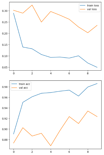
48/48 [==============================] - 28s 563ms/step - loss: 0.2891 - accuracy: 0.8908 - val_loss: 0.3023 - val_accuracy: 0.8737
Epoch 2/10
48/48 [==============================] - 19s 388ms/step - loss: 0.1395 - accuracy: 0.9507 - val_loss: 0.2896 - val_accuracy: 0.9026
Epoch 3/10
48/48 [==============================] - 19s 386ms/step - loss: 0.1318 - accuracy: 0.9612 - val_loss: 0.3254 - val_accuracy: 0.8868
Epoch 4/10
48/48 [==============================] - 19s 389ms/step - loss: 0.1064 - accuracy: 0.9678 - val_loss: 0.2501 - val_accuracy: 0.8921
Epoch 5/10
48/48 [==============================] - 19s 401ms/step - loss: 0.0935 - accuracy: 0.9691 - val_loss: 0.2970 - val_accuracy: 0.8684
Epoch 6/10
48/48 [==============================] - 19s 397ms/step - loss: 0.0952 - accuracy: 0.9717 - val_loss: 0.2806 - val_accuracy: 0.8974
Epoch 7/10
48/48 [==============================] - 19s 402ms/step - loss: 0.0905 - accuracy: 0.9737 - val_loss: 0.2625 - val_accuracy: 0.9237
Epoch 8/10
48/48 [==============================] - 19s 386ms/step - loss: 0.1007 - accuracy: 0.9625 - val_loss: 0.2284 - val_accuracy: 0.9105
Epoch 9/10
48/48 [==============================] - 19s 395ms/step - loss: 0.0687 - accuracy: 0.9796 - val_loss: 0.2028 - val_accuracy: 0.9342
Epoch 10/10
48/48 [==============================] - 21s 429ms/step - loss: 0.0497 - accuracy: 0.9862 - val_loss: 0.2356 - val_accuracy: 0.9237
Let’s plot training/validation accuracy and loss vs epochs
# plot the loss
plt.plot(r.history['loss'], label='train loss')
#plot the val_loss function
plt.plot(r.history['val_loss'], label='val loss')
plt.legend()
plt.show()

# plot the accuracy
plt.plot(r.history['accuracy'], label='train acc')
#plot the val_accuracy score
plt.plot(r.history['val_accuracy'], label='val acc')
plt.legend()
plt.show()
plt.savefig('AccVal_acc')
Test Data Predictions
Let’s use the above model to predict our test data
predictions = model.predict(test_dataset)
predictions = np.round(predictions)
Output:
12/12 [==============================] – 1s 88ms/step
Let’s invoke the image prediction and plotting function
def predictImage(filename):
#create a varibale and load_image with target_size
img1 = image.load_img(filename,target_size=(150,150))
#Let's visualize it using the matplotlib
plt.imshow(img1)
#Create y variable to covert the image into arrys
Y = image.img_to_array(img1)
#Expand the shape of an array.
#Insert a new axis that will appear at the axis position in the expanded array shape.
X = np.expand_dims(Y,axis=0)
#Predict the the test dataset
val = model.predict(X)
print(val)
#create condition to for predict the labels
if val == 1:
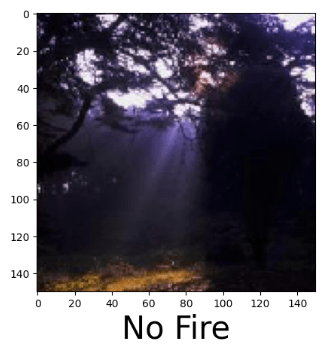
plt.xlabel("No Fire",fontsize=30)
elif val == 0:
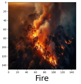
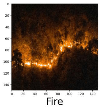
plt.xlabel("Fire",fontsize=30)
Let’s look at a few randomly selected test and public-domain forest fire images below:
predictImage(r'YOURPATH\Dataset\Testing\fire\abc003.jpg')

predictImage(r'YOURPATH\Dataset\Testing\nofire\abc195.jpg')
predictImage(r'YOURPATH\wildfires_fire6.jpg')

predictImage(r'YOURPATH\wildfires_fire5.jpg')

predictImage(r'YOURPATH\wildfires_fire4.jpg')

predictImage(r'YOURPATH\wildfires_fire3.jpg')
predictImage(r'YOURPATH\wildfires_fire2.jpg')
predictImage(r'YOURPATH\wildfires_fire1.jpg')

predictImage(r'YOURPATH\wildfires_fire0.jpg')

Summary
- Implementing the TensorFlow CNN can detect fire images with a high degree of accuracy and speed.
- The automated AI/DL forest fire detection algorithm has the potential to offer valuable insights to policymakers and authorities, supporting sustainable land-use planning and effective risk management practices.
Explore More
- Towards Optimized ML Wildfire Prediction
- ML/AI Wildfire Prediction using Remote Sensing Data
- ML/AI Wildfire Prediction
- Nonprofit
References
- Fire and smoke detection with Keras and Deep Learning
- Forest Fire Susceptibility Modeling Using a Convolutional Neural Network for Yunnan Province of China
- Computationally Efficient Wildfire Detection Method Using a Deep Convolutional Network Pruned via Fourier Analysis
- Forest Fire Prediction with Artificial Neural Network (Part 1)
- Prediction of Wildfire Using Machine Learning
- Forest Fire Detection-Prediction/ALL PROCESS
- Machine learning for wildfire classification: Exploring blackbox, eXplainable, symbolic, and SMOTE methods


Make a one-time donation
Make a monthly donation
Make a yearly donation
Choose an amount
Or enter a custom amount
Your contribution is appreciated.
Your contribution is appreciated.
Your contribution is appreciated.
DonateDonate monthlyDonate yearly
Leave a comment