Robust Fake News Detection: NLP Algorithms for Deep Learning and Supervised ML in Python

Featured Image via Canva

• The problem of Fake News has been affecting the world on a large scale because of the wide adoption of online social media platforms.
• In this project, we will classify text-based fake news from real news using AI-powered content-based NLP procedures.
• The ultimate goal is to create a robust fake news detector system in Python by implementing and comparing some common Deep Learning (DL), Supervised ML, and NLP algorithms.
• The proposed hybrid framework consists of the following steps, as shown below:
• Load news title & text, perform Exploratory Data Analysis (EDA), and NLP (stop word removal, tokenization, etc.)
• Perform multi-model training, testing, and X-validation by invoking several DL and supervised ML binary classifiers
• Select the best performing classification model by comparing several DL/ML performance metrics (KPIs)
• The entire E2E pipeline is refined if KPIs are not satisfactory in terms of the model bias-variance trade-off
• Otherwise, we export classified fake and real news.

• The Kaggle dataset will be used for the experiment; it is comprised of both false and true news.  

Input Dataset

Let’s set the working directory YOURPATH

import os
os.chdir(‘YOURPATH’)
os. getcwd()

and import the following libraries

import pandas as pd
import matplotlib.pyplot as plt
import numpy as np
import tensorflow as tf
import re
from tensorflow.keras.preprocessing.text import Tokenizer
import tensorflow as tf
from sklearn.metrics import accuracy_score
from sklearn.model_selection import train_test_split
from sklearn.metrics import accuracy_score, confusion_matrix, precision_score, recall_score
import seaborn as sns
plt.style.use(‘ggplot’)

Let’s read the input data

fake_df = pd.read_csv(‘Fake.csv’)
real_df = pd.read_csv(‘True.csv’)

and perform labeling of the target variable

fake_df[‘class’] = 0
real_df[‘class’] = 1

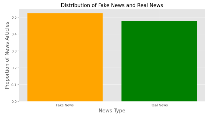
Let’s plot the Proportion of News Articles

total_len = len(fake_df) + len(real_df)
plt.figure(figsize=(10, 5))
plt.bar(‘Fake News’, len(fake_df) / total_len, color=’orange’)
plt.bar(‘Real News’, len(real_df) / total_len, color=’green’)
plt.title(‘Distribution of Fake News and Real News’, size=15)
plt.xlabel(‘News Type’, size=15)
plt.ylabel(‘Proportion of News Articles’, size=15)

Let’s perform text concatenation, define features and targets, and train/test data splitting with test_size=0.30

news_df = pd.concat([fake_df, real_df], ignore_index=True, sort=False)
news_df[‘text’] = news_df[‘title’] + news_df[‘text’]
news_df.drop(‘title’, axis=1, inplace=True)

features = news_df[‘text’]
targets = news_df[‘class’]

X_train, X_test, y_train, y_test = train_test_split(features, targets, test_size=0.30, random_state=42)

Let’s normalize our train and test feature data

def normalize(data):
normalized = []
for i in data:
i = i.lower()
# get rid of urls
i = re.sub(‘https?://\S+|www.\S+’, ”, i)
# get rid of non words and extra spaces
i = re.sub(‘\W’, ‘ ‘, i)
i = re.sub(‘\n’, ”, i)
i = re.sub(‘ +’, ‘ ‘, i)
i = re.sub(‘^ ‘, ”, i)
i = re.sub(‘ $’, ”, i)
normalized.append(i)
return normalized

X_train = normalize(X_train)
X_test = normalize(X_test)

Let’s tokenize the text into vectors

max_vocab = 10000
tokenizer = Tokenizer(num_words=max_vocab)
tokenizer.fit_on_texts(X_train)

X_train = tokenizer.texts_to_sequences(X_train)
X_test = tokenizer.texts_to_sequences(X_test)

and create the input data for our DL algorithm below

X_train = tf.keras.preprocessing.sequence.pad_sequences(X_train, padding=’post’, maxlen=256)
X_test = tf.keras.preprocessing.sequence.pad_sequences(X_test, padding=’post’, maxlen=256)

Deep Learning

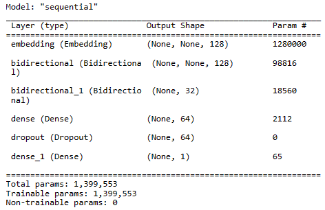
Let’s implement fake news detection using TF RNN:

model = tf.keras.Sequential([
tf.keras.layers.Embedding(max_vocab, 128),
tf.keras.layers.Bidirectional(tf.keras.layers.LSTM(64, return_sequences=True)),
tf.keras.layers.Bidirectional(tf.keras.layers.LSTM(16)),
tf.keras.layers.Dense(64, activation=’relu’),
tf.keras.layers.Dropout(0.5),
tf.keras.layers.Dense(1)
])

model.summary()

Let’s compile and run the above model

early_stop = tf.keras.callbacks.EarlyStopping(monitor=’val_loss’, patience=2, restore_best_weights=True)
model.compile(loss=tf.keras.losses.BinaryCrossentropy(from_logits=True),
optimizer=tf.keras.optimizers.Adam(1e-4),
metrics=[‘accuracy’])

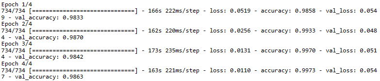
history = model.fit(X_train, y_train, epochs=4,validation_split=0.3, batch_size=30, shuffle=True, callbacks=[early_stop])

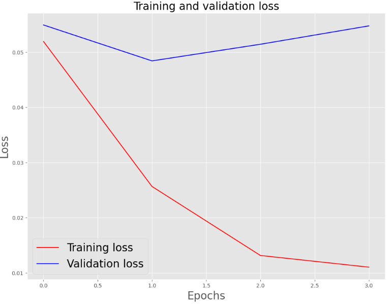
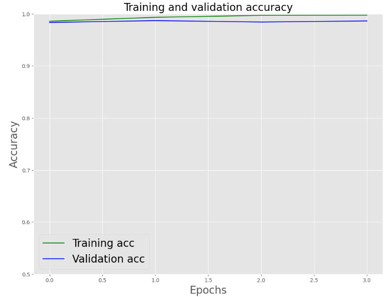
Let’s plot the training and validation loss/accuracy vs epochs

history_dict = history.history

acc = history_dict[‘accuracy’]
val_acc = history_dict[‘val_accuracy’]
loss = history_dict[‘loss’]
val_loss = history_dict[‘val_loss’]
epochs = history.epoch

plt.figure(figsize=(12,9))
plt.plot(epochs, loss, ‘r’, label=’Training loss’)
plt.plot(epochs, val_loss, ‘b’, label=’Validation loss’)
plt.title(‘Training and validation loss’, size=20)
plt.xlabel(‘Epochs’, size=20)
plt.ylabel(‘Loss’, size=20)
plt.legend(prop={‘size’: 20})
plt.show()

plt.figure(figsize=(12,9))
plt.plot(epochs, acc, ‘g’, label=’Training acc’)
plt.plot(epochs, val_acc, ‘b’, label=’Validation acc’)
plt.title(‘Training and validation accuracy’, size=20)
plt.xlabel(‘Epochs’, size=20)
plt.ylabel(‘Accuracy’, size=20)
plt.legend(prop={‘size’: 20})
plt.ylim((0.5,1))
plt.show()

Let’s evaluate our model on the test data

model.evaluate(X_test, y_test)

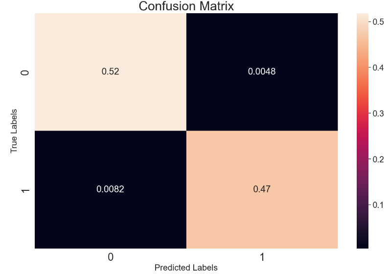
421/421 [====] – 20s 49ms/step – loss: 0.0482 – accuracy: 0.9870

[0.04822045937180519, 0.9870081543922424]

Let’s run our predictions on X_test

pred = model.predict(X_test)

binary_predictions = []

for i in pred:
if i >= 0.5:
binary_predictions.append(1)
else:
binary_predictions.append(0)

421/421 [==============================] – 22s 50ms/step

Let’s check the accuracy, precision, and recall of the test dataset

print(‘Accuracy on testing set:’, accuracy_score(binary_predictions, y_test))
print(‘Precision on testing set:’, precision_score(binary_predictions, y_test))
print(‘Recall on testing set:’, recall_score(binary_predictions, y_test))

Accuracy on testing set: 0.9870081662954714

Precision on testing set: 0.9899670794795422

Recall on testing set: 0.9827264239028944

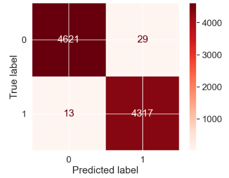
Let’s plot the RNN confusion matrix

matrix = confusion_matrix(binary_predictions, y_test, normalize=’all’)
plt.figure(figsize=(16, 10))
ax= plt.subplot()
sns.set(font_scale=1.8)
sns.heatmap(matrix, annot=True, ax = ax)

ax.set_xlabel(‘Predicted Labels’, size=20)
ax.set_ylabel(‘True Labels’, size=20)
ax.set_title(‘Confusion Matrix’, size=30)
ax.xaxis.set_ticklabels([0,1], size=25)
ax.yaxis.set_ticklabels([0,1], size=25)

We can also implement the DL fake news detection using the pyTorch LSTM approach with the test accuracy of 99.5%. See Appendix A.

Supervised ML

Let’s compare several supervised ML algorithms. In principle, we can take only some samples of the fake news dataset due to the memory and RAM issues. Anyways, our final goal is to create a predictive system.

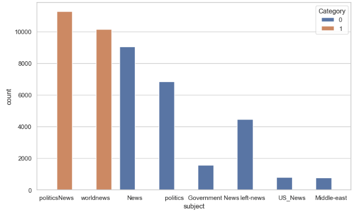
First, let’s invoke EDA with seaborn and nltk visualizations

import pandas as pd
import numpy as np
import matplotlib.pyplot as plt
import seaborn as sns
true = pd.read_csv(“True.csv”)
fake = pd.read_csv(“Fake.csv”)

true[‘Category’] = 1
fake[‘Category’] = 0
news = pd.concat([true,fake])

plt.figure(figsize=(10,6))
sns.set(font_scale=3)
sns.set(style= ‘whitegrid’)
count = sns.countplot(x=’subject’, hue=’Category’, data=news)

Let’s plot the word clouds of fake and real news:

news[‘texts’] = news[‘text’]+ ” ” +news[‘title’]

y = news[“Category”]
x = news[“texts”]

import nltk
import re
import string
nltk.download(‘punkt’)

from nltk.corpus import stopwords
from wordcloud import WordCloud, STOPWORDS, ImageColorGenerator

nltk.download(‘stopwords’)
stemmer = nltk.SnowballStemmer(‘english’)
stopword = set(stopwords.words(‘english’))

def clean(text):
text = str(text).lower()
text = re.sub(‘[.?]’, ”, text) text = re.sub(‘https?://\S+|www.\S+’, ”, text) text = re.sub(‘<.?>+’, ”, text)
text = re.sub(‘[%s]’ % re.escape(string.punctuation), ”, text)
text = re.sub(‘\n’, ”, text)
text = re.sub(‘\w\d\w‘, ”, text)
text = [word for word in text.split(‘ ‘) if word not in stopword]
text=” “.join(text)
text = [stemmer.stem(word) for word in text.split(‘ ‘)]
text=” “.join(text)
return text

x_clean = x.apply(clean)
fake_text = fake[‘text’]+ ” ” +fake[‘title’]
true_text = true[‘text’]+ ” ” +true[‘title’]

fake_clean = fake_text.apply(clean)
true_clean = true_text.apply(clean)
ftext = ” “.join(i for i in fake.text)
ttext = ” “.join(i for i in true.text)

• Fake News

from wordcloud import WordCloud, STOPWORDS
import matplotlib.pyplot as plt

wordcloud = WordCloud(stopwords=STOPWORDS, background_color=”white”).generate(ftext)
plt.figure(figsize=(15, 10))
plt.imshow(wordcloud, interpolation=’bilinear’)
plt.axis(“off”)
plt.show()

• Real News

wordcloud = WordCloud(stopwords=STOPWORDS, background_color=”white”).generate(ttext)
plt.figure(figsize=(15, 10))
plt.imshow(wordcloud, interpolation=’bilinear’)
plt.axis(“off”)
plt.show()

Let’s invoke TfidfVectorizer to transform text into numerical arrays

from sklearn.feature_extraction.text import TfidfVectorizer
from sklearn.model_selection import train_test_split
from sklearn.naive_bayes import MultinomialNB
from sklearn.metrics import accuracy_score, classification_report, confusion_matrix
X_train, X_test, y_train, y_test = train_test_split(x_clean, y, test_size=0.2, random_state=42)

vectorizer = TfidfVectorizer()
X_train_vectorized = vectorizer.fit_transform(X_train)
X_test_vectorized = vectorizer.transform(X_test)

classifier = MultinomialNB()
classifier.fit(X_train_vectorized, y_train)
y_pred = classifier.predict(X_test_vectorized)
accuracy = accuracy_score(y_test, y_pred)

Let’s check the accuracy score and plot the confusion matrix of the above classifier

print(f”Accuracy: {accuracy:.2f}”)

Accuracy: 0.94

from sklearn.metrics import confusion_matrix
from sklearn.metrics import ConfusionMatrixDisplay

cnf_matrix = confusion_matrix(y_test, y_pred)
disp = ConfusionMatrixDisplay(confusion_matrix=cnf_matrix, display_labels= classifier.classes_)
disp.plot(cmap=plt.cm.Blues)

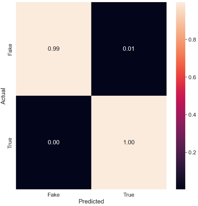
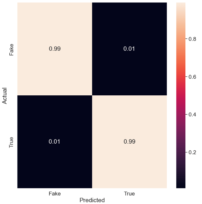
Let’s plot the normalized confusion matrix of MultinomialNB()

target_names=[‘Fake’,’True’]
sns.set(font_scale=1.5)
cmn = cnf_matrix .astype(‘float’) / cnf_matrix.sum(axis=1)[:, np.newaxis]
fig, ax = plt.subplots(figsize=(10,10))
sns.heatmap(cmn, annot=True, fmt=’.2f’, xticklabels=target_names, yticklabels=target_names)
plt.ylabel(‘Actual’)
plt.xlabel(‘Predicted’)
plt.show(block=False)

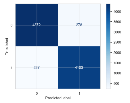
Let’s look at the SVC classifier

from sklearn.svm import SVC

model = SVC(kernel=’linear’, C=1.0)
model.fit(X_train_vectorized, y_train)

y_svm_pred = model.predict(X_test_vectorized)
accuracy = accuracy_score(y_test, y_svm_pred)
print(“Accuracy:”, accuracy)

Accuracy: 0.9953229398663697

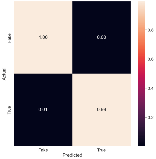
The SVC confusion matrix is as follows

cnf_matrix = confusion_matrix(y_test, y_svm_pred)
disp = ConfusionMatrixDisplay(confusion_matrix=cnf_matrix, display_labels= classifier.classes_)
disp.plot(cmap=plt.cm.Reds)

The normalized SVC confusion matrix is given by

target_names=[‘Fake’,’True’]
sns.set(font_scale=1.5)
cmn = cnf_matrix .astype(‘float’) / cnf_matrix.sum(axis=1)[:, np.newaxis]
fig, ax = plt.subplots(figsize=(10,10))
sns.heatmap(cmn, annot=True, fmt=’.2f’, xticklabels=target_names, yticklabels=target_names)
plt.ylabel(‘Actual’)
plt.xlabel(‘Predicted’)
plt.show(block=False)

The same confusion matrix is obtained with the help of GradientBoostingClassifier, RidgeClassifier and SGDClassifier.

Let’s consider AdaBoostClassifier

from sklearn.ensemble import AdaBoostClassifier
model = AdaBoostClassifier(random_state=42)
model.fit(X_train_vectorized, y_train)

y_pred = model.predict(X_test_vectorized)
accuracy = accuracy_score(y_test, y_pred)
print(“Accuracy:”, accuracy)

Accuracy: 0.9952115812917595

The normalized confusion matrix of AdaBoostClassifier is

cnf_matrix = confusion_matrix(y_test, y_pred)
target_names=[‘Fake’,’True’]
sns.set(font_scale=1.5)
cmn = cnf_matrix .astype(‘float’) / cnf_matrix.sum(axis=1)[:, np.newaxis]
fig, ax = plt.subplots(figsize=(10,10))
sns.heatmap(cmn, annot=True, fmt=’.2f’, xticklabels=target_names, yticklabels=target_names)
plt.ylabel(‘Actual’)
plt.xlabel(‘Predicted’)
plt.show(block=False)

Let’s look at MLPClassifier

from sklearn.neural_network import MLPClassifier
model = MLPClassifier()
model.fit(X_train_vectorized, y_train)

y_pred = model.predict(X_test_vectorized)
accuracy = accuracy_score(y_test, y_pred)
print(“Accuracy:”, accuracy)

Accuracy: 0.9935412026726058

The MLP normalized confusion matrix is

cnf_matrix = confusion_matrix(y_test, y_pred)
target_names=[‘Fake’,’True’]
sns.set(font_scale=1.5)
cmn = cnf_matrix .astype(‘float’) / cnf_matrix.sum(axis=1)[:, np.newaxis]
fig, ax = plt.subplots(figsize=(10,10))
sns.heatmap(cmn, annot=True, fmt=’.2f’, xticklabels=target_names, yticklabels=target_names)
plt.ylabel(‘Actual’)
plt.xlabel(‘Predicted’)
plt.show(block=False)

Let’s consider DecisionTreeClassifier

from sklearn.tree import DecisionTreeClassifier
model = DecisionTreeClassifier()
model.fit(X_train_vectorized, y_train)

y_pred = model.predict(X_test_vectorized)
accuracy = accuracy_score(y_test, y_pred)
print(“Accuracy:”, accuracy)

Accuracy: 0.9968819599109131

The normalized confusion matrix of DecisionTreeClassifier is

cnf_matrix = confusion_matrix(y_test, y_pred)
target_names=[‘Fake’,’True’]
sns.set(font_scale=1.5)
cmn = cnf_matrix .astype(‘float’) / cnf_matrix.sum(axis=1)[:, np.newaxis]
fig, ax = plt.subplots(figsize=(10,10))
sns.heatmap(cmn, annot=True, fmt=’.2f’, xticklabels=target_names, yticklabels=target_names)
plt.ylabel(‘Actual’)
plt.xlabel(‘Predicted’)
plt.show(block=False)

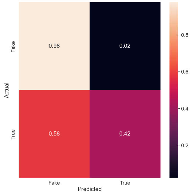
Let’s look at KNeighborsClassifier

from sklearn.neighbors import KNeighborsClassifier
model = KNeighborsClassifier()
model.fit(X_train_vectorized, y_train)

y_pred = model.predict(X_test_vectorized)
accuracy = accuracy_score(y_test, y_pred)
print(“Accuracy:”, accuracy)

Accuracy: 0.7082405345211581

The KNN normalized confusion matrix is

cnf_matrix = confusion_matrix(y_test, y_pred)
target_names=[‘Fake’,’True’]
sns.set(font_scale=1.5)
cmn = cnf_matrix .astype(‘float’) / cnf_matrix.sum(axis=1)[:, np.newaxis]
fig, ax = plt.subplots(figsize=(10,10))
sns.heatmap(cmn, annot=True, fmt=’.2f’, xticklabels=target_names, yticklabels=target_names)
plt.ylabel(‘Actual’)
plt.xlabel(‘Predicted’)
plt.show(block=False)

Let’s consider RandomForestClassifier

from sklearn.ensemble import RandomForestClassifier
model = RandomForestClassifier()
model.fit(X_train_vectorized, y_train)

y_pred = model.predict(X_test_vectorized)
accuracy = accuracy_score(y_test, y_pred)
print(“Accuracy:”, accuracy)

Accuracy: 0.9903118040089087

As with MLP, the RFC normalized confusion matrix is

cnf_matrix = confusion_matrix(y_test, y_pred)
target_names=[‘Fake’,’True’]
sns.set(font_scale=1.5)
cmn = cnf_matrix .astype(‘float’) / cnf_matrix.sum(axis=1)[:, np.newaxis]
fig, ax = plt.subplots(figsize=(10,10))
sns.heatmap(cmn, annot=True, fmt=’.2f’, xticklabels=target_names, yticklabels=target_names)
plt.ylabel(‘Actual’)
plt.xlabel(‘Predicted’)
plt.show(block=False)

The same confusion matrix is obtained using other classifiers such as LogisticRegression.

A few classifiers (e.g. QuadraticDiscriminantAnalysis) yield the following error

TypeError: A sparse matrix was passed, but dense data is required. Use X.toarray() to convert to a dense numpy array.

Conclusions

• This study can help us better understand the possibilities for applying AI and NLP to address the important issue of fake news.
• To determine whether you can get better outcomes, we considered different algorithms and strategies.

• Specifically, we implemented and tested both Deep Learning (DL) and various supervised ML (linear, ensemble, trees, MLP, etc.) models. We used these models to detect whether the specific news is fake or not.
• The DL detection model was built using TensorFlow RNN. One could also invoke pyTorch LSTM, as shown in Appendix A.
• We followed the following steps: Importing Libraries and dataset; Preprocessing Dataset; Generating Word Embeddings; Model Architecture; Model Evaluation and Prediction.
• We can see our DL/ML models are performing very well even on the evaluation data with ACC~99% and FP, FN ~ 1%, excluding KNN.
• We also tested the Streamlit web app for the task of fake news detection, as explained in Appendix B.

• This approach may also be used in other classification techniques such as spam detection, sentiment analysis, and prediction of loan eligibility, among other things.

References

• Fake News Detection Using Machine Learning and Deep Learning Algorithms
• Fake News Classification using transformer based enhanced LSTM and BERT
• Predicting Fake News using NLP and Machine Learning | Scikit-Learn | GloVe | Keras | LSTM
• Fake News Classification Using Deep Learning
• Fake News Detection using Machine Learning | Fake News Detection Project | Data Magic
• Detecting Fake News with Python and Machine Learning
• Fake news detection using machine learning | Learn with Simple Coding Exercises | kandi tutorial
• Fake News Detection using Machine Learning
• How To Detect Fake News Using Ensemble Learning
• Fake News Detection with Python
• Fake News Classification Based on Content Level Features

Appendix A: PyTorch LSTM

Let’s import the key libraries

import numpy as np # linear algebra
import pandas as pd # data processing, CSV file I/O (e.g. pd.read_csv)
import os
import random
import re
import numpy as np
import pandas as pd
import torch
from torchtext.data.utils import get_tokenizer
from torchtext.vocab import build_vocab_from_iterator
from nltk.corpus import stopwords
from torch.utils.data import TensorDataset, DataLoader
import torch.nn as nn
from torch.nn import CrossEntropyLoss
from torch.optim import Adam
from torch.optim.lr_scheduler import ReduceLROnPlateau
from sklearn import metrics
from sklearn.utils.class_weight import compute_class_weight
from tqdm import tqdm
import torch.nn.functional as F
import matplotlib.pyplot as plt

pd.options.mode.chained_assignment = None

Let’s define the test hyperparameters
vocab_size = 160_000
embedding_dim = 300
hidden_dim = 128
n_layers = 2
seq_len = 2000
learning_rate = 0.0025
max_epochs = 2
batch_size = 40

Let’s perform the following data editing steps:

• Read data
  real = pd.read_csv(“True.csv”)
  fake = pd.read_csv(“Fake.csv”)

• Create labels
  real[“label”] = 1
  fake[“label”] = 0

• Combine and shuffle the data
  combined = pd.concat([fake, real], axis=0)
  combined = combined.sample(frac=1).reset_index(drop=True)

• Split dataset into the train, validation and test sets with the ratio of 70-15-15
  train = combined[:int(0.7 * len(combined))]
  val = combined[int(0.7 * len(combined)):int(0.85 * len(combined))]
  test = combined[int(0.85 * len(combined)):]

Let’s check the shapes

train.shape, val.shape, test.shape

((31428, 5), (6735, 5), (6735, 5))

Let’s define the following objects

def build_vocabulary():
train_iterator = list(zip(train[‘text’], train[‘label’]))
tokenizer = get_tokenizer(“basic_english”)

def tokenizer_fn(data_iterator):
    for text, _ in data_iterator:
        yield tokenizer(text)

vocab = build_vocab_from_iterator(tokenizer_fn(train_iterator), specials=["<unk>"])
vocab.set_default_index(vocab["<unk>"])

return vocab, tokenizer

def clean_text(dataframe):
dataframe[“text”] = dataframe[“subject”] + ” ” + dataframe[“title”] + ” ” + dataframe[“text”]

del dataframe['title']
del dataframe['subject']
del dataframe['date']

stop_words = list(set(stopwords.words('english')))

def _process_text(text):
    text = text.lower()
    text = " ".join([word for word in text.split() if word not in stop_words])
    text = re.sub(r"[^\w\s]", '', text)
    return text

dataframe['text'] = dataframe['text'].apply(_process_text)

return dataframe

def tokenize_text(dataframe, vocab, tokenizer):
dataframe[“text”] = dataframe[“text”].apply(lambda x: np.array(vocab(tokenizer(x)), dtype=np.int64))
return dataframe[[‘text’, ‘label’]]

def pad_tokens(dataframe, vocab, max_len):
dataframe[‘text’] = dataframe[‘text’].apply(
lambda x: np.pad(x, (0, max(0, max_len – len(x))), ‘constant’, constant_values=vocab[“”]))
dataframe[“text”] = dataframe[“text”].apply(lambda x: x[:max_len])
return dataframe

def create_dataloader(dataframe, vocab, tokenizer, seq_len, batch_size):
dataframe = clean_text(dataframe)
dataframe = tokenize_text(dataframe, vocab, tokenizer)
dataframe = pad_tokens(dataframe=dataframe, vocab=vocab, max_len=seq_len)

dataset = TensorDataset(
    torch.from_numpy(np.vstack(dataframe["text"].values)),
    torch.from_numpy(dataframe["label"].values)
)

return DataLoader(
    dataset,
    batch_size=batch_size,
    num_workers=1
)

vocab, tokenizer = build_vocabulary()

train_dataloader = create_dataloader(
dataframe=train,
vocab=vocab,
tokenizer=tokenizer,
seq_len=seq_len,
batch_size=batch_size
)

val_dataloader = create_dataloader(
dataframe=val,
vocab=vocab,
tokenizer=tokenizer,
seq_len=seq_len,
batch_size=batch_size
)

test_dataloader = create_dataloader(
dataframe=test,
vocab=vocab,
tokenizer=tokenizer,
seq_len=seq_len,
batch_size=batch_size
)

class Trainer:
def init(self, model, train_dataloader, val_dataloader, test_dataloader, device, criterion, optimizer):
self.model = model
self.train_dataloader = train_dataloader
self.val_dataloader = val_dataloader
self.test_dataloader = test_dataloader
self.device = device
self.criterion = criterion
self.optimizer = optimizer

def train(self, current_epoch_nr):
    self.model.train()

    num_batches = len(self.train_dataloader)

    preds = []
    targets = []
    correct = 0
    running_loss = 0.0
    items_processed = 0

    loop = tqdm(enumerate(self.train_dataloader), total=num_batches)
    for idx, (x, y) in loop:
        x = x.to(self.device)
        y = y.to(self.device)

        y_hat = self.model(x)

        loss = self.criterion(y_hat, y)
        loss.backward()

        self.optimizer.step()
        self.optimizer.zero_grad()

        running_loss += loss.item()

        _, predicted = y_hat.max(1)
        items_processed += y.size(0)
        correct += predicted.eq(y).sum().item()

        targets.extend(y.detach().cpu().numpy().flatten())
        preds.extend(predicted.detach().cpu().numpy().flatten())

        loop.set_description(f'Epoch {current_epoch_nr + 1}')
        loop.set_postfix(train_acc=round(correct / items_processed, 4),
                         train_loss=round(running_loss / items_processed, 4))

    train_auc = metrics.roc_auc_score(targets, preds)
    train_accuracy = correct / items_processed
    train_loss = running_loss / items_processed

    return train_auc, train_accuracy, train_loss

def evaluate(self, current_epoch_nr, scheduler):
    self.model.eval()

    num_batches = len(self.val_dataloader)

    preds = []
    targets = []
    correct = 0
    running_loss = 0.0
    items_processed = 0

    with torch.no_grad():
        loop = tqdm(enumerate(self.val_dataloader), total=num_batches)
        for idx, (x, y) in loop:
            x = x.to(self.device)
            y = y.to(self.device)

            y_hat = self.model(x)

            loss = self.criterion(y_hat, y)

            running_loss += loss.item()

            _, predicted = y_hat.max(1)
            items_processed += y.size(0)
            correct += predicted.eq(y).sum().item()

            targets.extend(y.detach().cpu().numpy().flatten())
            preds.extend(predicted.detach().cpu().numpy().flatten())

            loop.set_description(f'Epoch {current_epoch_nr + 1}')
            loop.set_postfix(val_acc=round(correct / items_processed, 4),
                             val_loss=round(running_loss / items_processed, 4))

    val_auc = metrics.roc_auc_score(targets, preds)
    validation_accuracy = correct / items_processed
    validation_loss = running_loss / num_batches

    scheduler.step(validation_accuracy)

    return val_auc, validation_accuracy, validation_loss

def test(self):
    self.model.eval()

    num_batches = len(self.test_dataloader)

    preds = []
    targets = []
    running_loss = 0.0
    correct = 0
    total = 0

    with torch.no_grad():
        loop = tqdm(enumerate(self.test_dataloader), total=num_batches)
        for idx, (x, y) in loop:
            x = x.to(self.device)
            y = y.to(self.device)

            y_hat = self.model(x)

            loss = self.criterion(y_hat, y)

            running_loss += loss.item()

            _, predicted = y_hat.max(1)
            total += y.size(0)
            correct += predicted.eq(y).sum().item()

            targets.extend(y.detach().cpu().numpy().flatten())
            preds.extend(predicted.detach().cpu().numpy().flatten())

            loop.set_description('Testing')
            loop.set_postfix(test_acc=round(correct / total, 4),
                             test_loss=round(running_loss / total, 4))

    test_auc = metrics.roc_auc_score(targets, preds)
    test_accuracy = correct / total
    test_loss = running_loss / num_batches

    return test_auc, test_accuracy, test_loss

class LSTM(nn.Module):
def init(self, vocab_size, embedding_dim, hidden_dim, n_layers, seq_len):
super(LSTM, self).init()
self.embedding = nn.Embedding(vocab_size, embedding_dim)
self.lstm = nn.LSTM(input_size=embedding_dim, hidden_size=hidden_dim, num_layers=n_layers, batch_first=True)
self.fc = nn.Linear(seq_len * hidden_dim, 2)

def forward(self, x):
    x = self.embedding(x)
    x, _ = self.lstm(x)
    x = torch.reshape(x, (x.size(0), -1,))
    x = self.fc(x)
    return F.log_softmax(x, dim=-1)

Let’s train and test the model

device = “cuda” # or cpu

model = LSTM(
vocab_size=vocab_size,
embedding_dim=embedding_dim,
hidden_dim=hidden_dim,
n_layers=n_layers,
seq_len=seq_len
).to(device)

class_weights = compute_class_weight(‘balanced’, classes=[0, 1], y=train[“label”])
class_weights = torch.tensor(class_weights, dtype=torch.float).to(device)

criterion = CrossEntropyLoss(weight=class_weights, reduction=”mean”)
optimizer = Adam(lr=learning_rate, params=model.parameters())
scheduler = ReduceLROnPlateau(optimizer, mode=”max”, factor=0.5, patience=2)

trainer = Trainer(
model=model,
train_dataloader=train_dataloader,
val_dataloader=val_dataloader,
test_dataloader=test_dataloader,
device=device,
criterion=criterion,
optimizer=optimizer
)

train_aucs = []
train_accs = []
train_losses = []

val_aucs = []
val_accs = []
val_losses = []

for epoch in range(max_epochs):
train_auc, train_accuracy, train_loss = trainer.train(current_epoch_nr=epoch)
train_aucs.append(train_auc)
train_accs.append(train_accuracy)
train_losses.append(train_loss)

val_auc, val_accuracy, val_loss = trainer.evaluate(current_epoch_nr=epoch, scheduler=scheduler)
val_aucs.append(val_auc)
val_accs.append(val_accuracy)
val_losses.append(val_loss)

test_auc, test_accuracy, test_loss = trainer.test()

Epoch 1: 100%| 786/786 [26:20<00:00, 2.01s/it,

train_acc=0.996, train_loss=0.0008

Epoch 2: 100%| 786/786 [55:27<00:00, 4.23s/it,

train_acc=0.998, train_loss=0.0005

The three validation plotting functions are

fig, axs = plt.subplots(1, 3, figsize=(12, 4))

axs[0].plot(train_aucs, label=’train’)
axs[0].plot(val_aucs, label=’val’)
axs[0].set_xlabel(‘Epochs’)
axs[0].set_title(‘AUC’)
axs[0].legend()

axs[1].plot(train_accs, label=’train’)
axs[1].plot(val_accs, label=’val’)
axs[1].set_xlabel(‘Epochs’)
axs[1].set_title(‘Accuracy’)
axs[1].legend()

axs[2].plot(train_losses, label=’train’)
axs[2].plot(val_losses, label=’val’)
axs[2].set_xlabel(‘Epochs’)
axs[2].set_title(‘Loss’)
axs[2].legend()

plt.tight_layout()
plt.show()

Appendix B: Streamlit App

Let’s create the Streamlit web app fakenews.py for the task of fake news detection with the input dataset fake_or_real_news.csv (titles only):

import pandas as pd
import numpy as np
from sklearn.feature_extraction.text import CountVectorizer
from sklearn.model_selection import train_test_split

from sklearn.ensemble import AdaBoostClassifier
model = AdaBoostClassifier(random_state=42)
data = pd.read_csv(“fake_or_real_news.csv”)

x = np.array(data[“title”])
y = np.array(data[“label”])

cv = CountVectorizer()
x = cv.fit_transform(x)
xtrain, xtest, ytrain, ytest = train_test_split(x, y, test_size=0.2, random_state=42)

model.fit(xtrain, ytrain)

import streamlit as st
st.title(“Fake News Detection System”)
def fakenewsdetection():
user = st.text_area(“Enter Any News Headline: “)
if len(user) < 1:
st.write(” “)
else:
sample = user
data = cv.transform([sample]).toarray()
a = model.predict(data)
st.title(a)
fakenewsdetection()

We run this app from the cmd prompt as follows

streamlit run fakenews.py