Supervised ML Room Occupancy IoT

Featured Photo via Canva

• The integration of occupancy detection IoT sensors with smart building ML management systems provides a foundation for smarter and more efficient decisions about space allocation in the workplace.
• In this post, we will compare most popular supervised ML binary classification techniques for room occupancy IoT monitoring.

• Based upon the overall model performance and previous studies, we have selected the following 14 scikit-learn classifiers: Logistic Regression (LR), Decision Tree (DT), Random Forest (RF), K-Nearest Neighbors (KNN), Naïve Bayes (NB), Support Vector Machine (SVC), Gradient Boosting (GB), Multi-Layer Perceptron (MLP), Ada Boosting (Ada), Linear Discriminant Analysis (LDA), Calibrated Classifier CV (CCCV), SGD Classifier (SGD), Extra Trees Classifier (ET), and Bagging Classifier (BC).

• Our objective is to show the QC analysis performed over the gathered IoT sensor data using ML is possible to determine and predict the room occupancy with high degree of certainty.
• Using the proposed ML IoT solution enables the transition to new normal office where desk sharing is at the center of hybrid work and empowers your employees with the choice of their preferred desk or space.

Table of Contents

1. About IoT Sensors
2. Input Kaggle Dataset
3. Exploratory Data Analysis
4. Training Multiple ML Models
5. ML Performance Summary
6. Conclusions
7. References

About IoT Sensors

• Occupancy monitoring IoT sensors are used for real-time occupancy detection in various places such as desks, phone booths, rooms, offices, hospitals or warehouses.
• Occupancy monitoring requires the deployment of IoT sensors that can reliably detect the presence of tenants in desks, offices, break-out areas, and other building spaces.
• Some examples of sensors are smart lighting sensors, cameras and people counting, blue tooth low energy solutions, infrared sensors, and ultrasonic sensors.

Input Kaggle Dataset

Let’s set the working directory

import os
os.chdir(‘YOURPATH’)
os. getcwd()

and import the following libraries

import seaborn as sns
import matplotlib.pyplot as plt
import plotly.express as px
import plotly.graph_objects as go

from tensorflow import keras
from tensorflow.keras import layers

from sklearn.model_selection import train_test_split

from sklearn.metrics import ConfusionMatrixDisplay
from sklearn.metrics import confusion_matrix

from sklearn.metrics import roc_auc_score

from sklearn.metrics import roc_curve
from sklearn.metrics import RocCurveDisplay
from sklearn.metrics import auc
from sklearn.metrics import accuracy_score
from sklearn.metrics import balanced_accuracy_score

from eli5.sklearn import PermutationImportance
from eli5.permutation_importance import get_score_importances

import tensorflow as tf

import numpy as np # linear algebra
import pandas as pd # data processing

Let’s read the input Kaggle dataset

raw_data = pd.read_csv(‘Occupancy.csv’)

and print the key information about the data

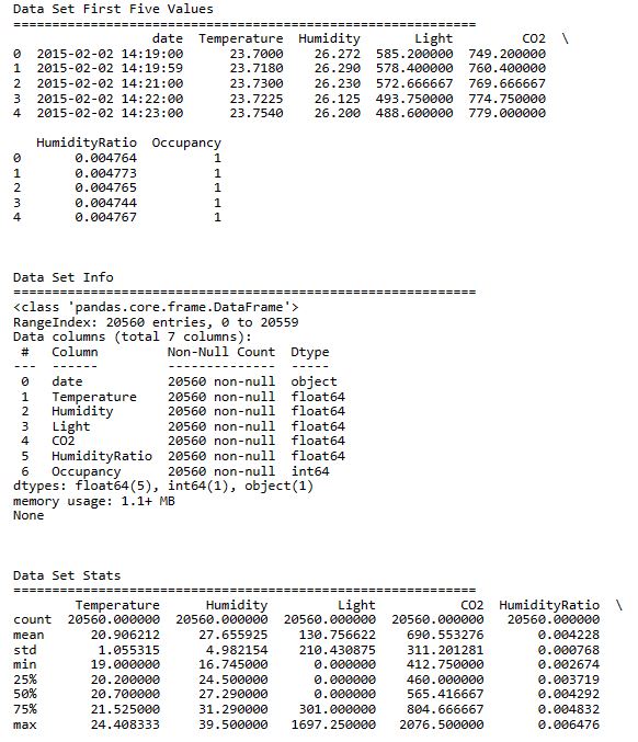
print(“Data Set First Five Values”)
print(60 * ‘=’)
print(raw_data.head())
print(‘\n\n’)

print(“Data Set Info”)
print(60 * ‘=’)
print(raw_data.info())
print(‘\n\n’)

print(“Data Set Stats”)
print(60 * ‘=’)
print(raw_data.describe())
print(‘\n\n’)

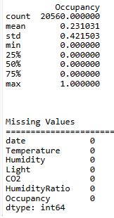
print(‘Missing Values’)
print(‘=’ * 60)
print(raw_data.isna().sum())

Exploratory Data Analysis

Let’s copy the data frame

df=raw_data.copy()

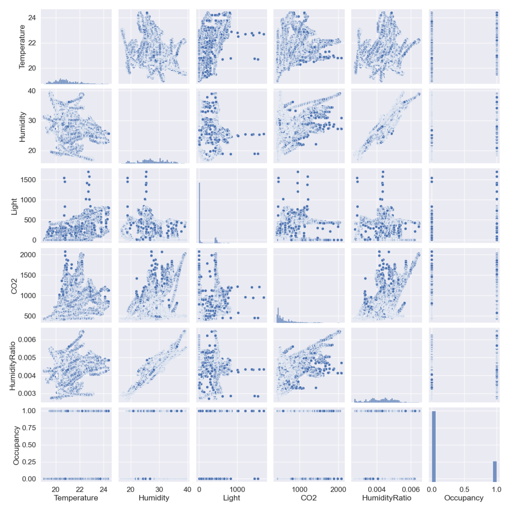
and plot the sns pairplot

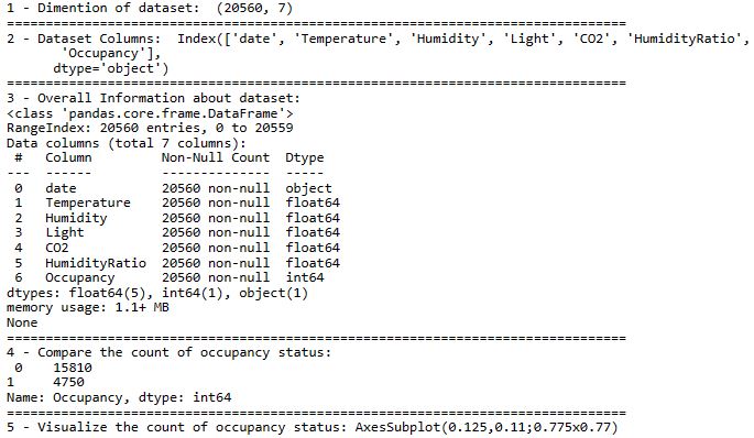
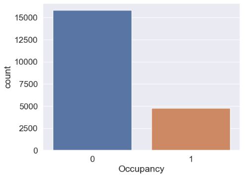
Let’s get some extra info about the dataset and visualize the count of occupancy status

print(“1 – Dimention of dataset: ” , df.shape)
print(80*”=”)

print(“2 – Dataset Columns: ” ,df.columns)
print(80*”=”)

print(“1 – Features of Dataset: ” , features)

print(80*”=”)

print(“3 – Overall Information about dataset: “)
print(df.info())
print(80*”=”)

print(“4 – Compare the count of occupancy status:\n”,df[“Occupancy”].value_counts())
print(80*”=”)

print(“5 – Visualize the count of occupancy status:”,sns.countplot(x=”Occupancy”, data=df))

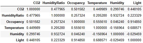
Let’s plot the correlation table and matrix of numerical variables

_, axes = plt.subplots(nrows=1, ncols=1, figsize=(8, 5))
numerical = list(set(df.columns)- {“date”})
corr_matrix = df[numerical].corr()
display(corr_matrix)

sns.heatmap(corr_matrix,ax=axes,annot=True);

plt.savefig(‘iotsnsnheatmap.png’)

Training Multiple ML Models

Let’s import the following libraries

import numpy as np
import matplotlib.pyplot as plt
import seaborn as sns
from sklearn import datasets, svm, metrics
from sklearn.model_selection import train_test_split
from sklearn.neural_network import MLPClassifier
from sklearn.metrics import classification_report,confusion_matrix
from sklearn.metrics import roc_auc_score
from sklearn.metrics import roc_curve
from sklearn.linear_model import LogisticRegression,Perceptron,SGDClassifier
from sklearn.tree import DecisionTreeClassifier
from sklearn.ensemble import RandomForestClassifier
from sklearn.neighbors import KNeighborsClassifier
from sklearn.naive_bayes import GaussianNB
from sklearn.svm import SVC
from sklearn.ensemble import GradientBoostingClassifier, AdaBoostClassifier,ExtraTreesClassifier,BaggingClassifier
from sklearn.discriminant_analysis import LinearDiscriminantAnalysis
from sklearn.calibration import CalibratedClassifierCV

and introduce the following two functions

def accuracy_vis(xtest, ytest, ypred, predit_proba,plotFlag):

cm = confusion_matrix(ytest, ypred)
sns.set(font_scale=1.4)
if plotFlag:
fig, (ax1, ax2) = plt.subplots(1, 2, figsize=(14,4))
x_axis_labels = [‘Actual Postive’, ‘Actual Negative’]
y_axis_labels = [‘Predicted Postive’, ‘Predicted Negative’]
sns.heatmap(cm, fmt=”.0f”, annot=True, linewidths=.5, ax=ax1,
cmap=”YlGnBu”, xticklabels=x_axis_labels)
ax1.set_yticklabels(y_axis_labels, rotation=0, ha=’right’)

 
    logit_roc_auc = roc_auc_score(ytest, ypred)
    fpr, tpr, thresholds = roc_curve(ytest, predit_proba[:,1])
    ax2.plot(fpr, tpr, label='ROC_AUC (area = {})'.format(round(logit_roc_auc,6)))
    ax2.plot([0, 1], [0, 1],'r--')
    ax2.set_xlim([0.0, 1.0])
    ax2.set_ylim([0.0, 1.05])
    ax2.set_xlabel('False Positive Rate')
    ax2.set_ylabel('True Positive Rate')
    ax2.legend()

    plt.show()
return(confusion_matrix(ytest, ypred).ravel())

def applyModel(df,selectedModel,plotFlag=True):

df2=df
X, Y = df2.iloc[:,1:-1], df2.iloc[:,-1]
X_train, X_test, Y_train, Y_test = train_test_split(X, Y, test_size=0.25, random_state=0)

modelTitle = selectedModel[0]
absTitle = selectedModel[1]
per = Perceptron()
model=""

if modelTitle == "Logistic Regression":
    model = LogisticRegression()

elif modelTitle == "DecisionTree":
    model = DecisionTreeClassifier()

elif modelTitle == "RandomForest":
    model = RandomForestClassifier(n_estimators= 10)

elif modelTitle == "K-Nearest Neighbors":
    model = KNeighborsClassifier(n_neighbors=int(np.sqrt(len(X_train))), metric= 'minkowski' ,p= 2)

elif modelTitle == "Naive Bayes":
    model = GaussianNB()

elif modelTitle == "Support Vector Machine":
    model = SVC(probability=True)

elif modelTitle == "Gradient Boosting":
    model = GradientBoostingClassifier()

elif modelTitle == "Ada Boosting":
    model = AdaBoostClassifier()

elif modelTitle == "Linear Discriminant Analysis":
    model = LinearDiscriminantAnalysis()

elif modelTitle == "Calibrated Classifier CV":
    model = CalibratedClassifierCV(per, cv=10, method='isotonic')

elif modelTitle == "SGD Classifier":
    model = SGDClassifier(loss='log_loss') 

elif modelTitle == "Extra Trees Classifier":
    model = ExtraTreesClassifier()  

elif modelTitle == "Bagging Classifier":
    model = BaggingClassifier()  


elif modelTitle == "Multi-Layer Perceptron":
    model = MLPClassifier(hidden_layer_sizes=(8,8,8), activation='relu', solver='adam', max_iter=500) 

if model != "":
    model.fit(X_train, Y_train)
    Y_pred, model_score, predit_proba = model.predict(X_test), model.score(X_test, Y_test), model.predict_proba(X_test)
    if plotFlag:
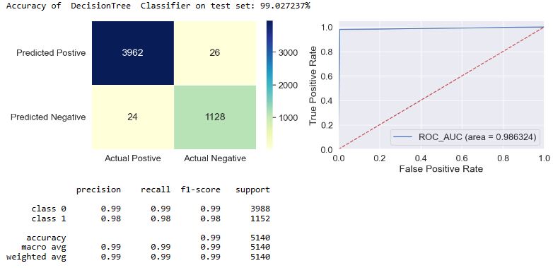
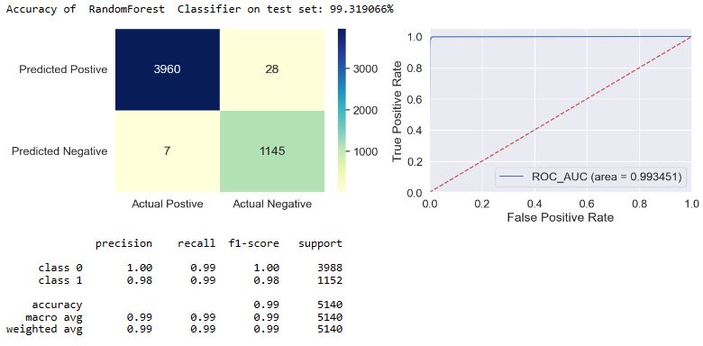
        print('Accuracy of ',modelTitle,' Classifier on test set: {:.6f}%'.format(model_score*100))

    tn, fp, fn, tp = accuracy_vis(X_test, Y_test, Y_pred, predit_proba,plotFlag)


    target_names = ['class 0', 'class 1']
    print(classification_report(Y_test, Y_pred, target_names=target_names))

    result.loc[absTitle] = [modelTitle, tn, fp, fn, tp, round(model_score*100, 6)]

Let’s use the above function to train and test our selected ML models

applyModel(df,[“Logistic Regression”,”LR”])

applyModel(df,[“DecisionTree”,”DT”])

applyModel(df,[“RandomForest”,”RF”])

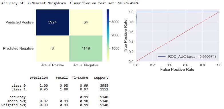
applyModel(df,[“K-Nearest Neighbors”,”KNN”])

applyModel(df,[“Naive Bayes”,”NB”])

applyModel(df,[“Support Vector Machine”,”SVC”])

applyModel(df,[“Gradient Boosting”,”GB”])

applyModel(df,[“Multi-Layer Perceptron”,”MLP”])

applyModel(df,[“Ada Boosting”,”Ada”])

applyModel(df,[“Linear Discriminant Analysis”,”LDA”])

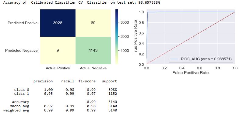
applyModel(df,[“Calibrated Classifier CV”,”CCCV”])

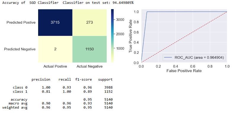
applyModel(df,[“SGD Classifier”,”SGD”])

applyModel(df,[“Extra Trees Classifier”,”ET”])

applyModel(df,[“Bagging Classifier”,”BC”])

ML Performance Summary

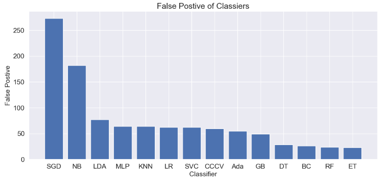
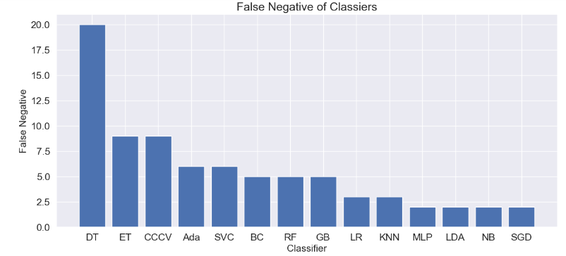
Let’s look at the summary table and the FP/FN bar plots

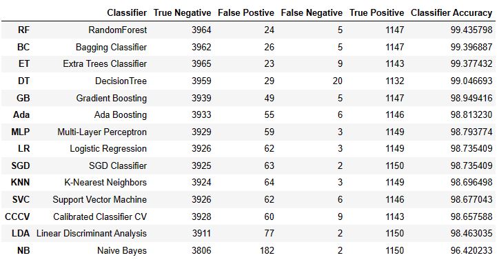
result.sort_values(‘Classifier Accuracy’, ascending=False)

Let’s create the sorted Pandas data frame from the two lists

Classifier = [“BC”, “ET”,”RF”,”DT”,”GB”,”Ada”, “LR”,”MLP”,”KNN”,”SVC”,”CCCV”,”LDA”,”NB”,”SGD”]

FP = [26,23,24,29,49,55,62,64,64,62,60,77,182,273]

FN = [5,9,5,20,5,6,3,2,3,6,9,2,2,2]

dfc = pd.DataFrame({“Classifier”:Classifier,
“False Postive”:FP,”False Negative”:FN})
dfc_sorted= dfc.sort_values(‘False Postive’,ascending=False)
dfcn_sorted= dfc.sort_values(‘False Negative’,ascending=False)

plt.figure(figsize=(14,6))

plt.bar(‘Classifier’, ‘False Postive’,data=dfc_sorted)
plt.xlabel(“Classifier”, size=15)
plt.ylabel(“False Postive”, size=15)
plt.title(“False Postive of Classiers”, size=18)
plt.savefig(“iot_fp_barplot.png”)

plt.figure(figsize=(14,6))

plt.bar(‘Classifier’, ‘False Negative’,data=dfcn_sorted)
plt.xlabel(“Classifier”, size=15)
plt.ylabel(“False Negative”, size=15)
plt.title(“False Negative of Classiers”, size=18)
plt.savefig(“iot_fn_barplot.png”)

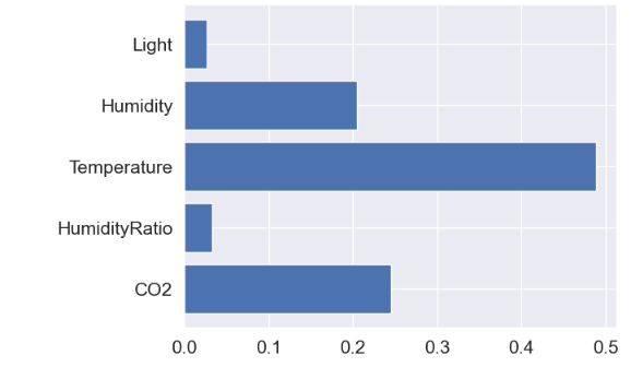
As an example, let’s compare the model features in terms of their dominance in the Random Forest Classifier

df2=df
X, Y = df2.iloc[:,1:-1], df2.iloc[:,-1]
X_train, X_test, Y_train, Y_test = train_test_split(X, Y, test_size=0.25, random_state=0)

model = RandomForestClassifier(n_estimators= 10)
model.fit(X_train, Y_train)
Y_pred, model_score, predit_proba = model.predict(X_test), model.score(X_test, Y_test), model.predict_proba(X_test)

model.feature_importances_

array([0.24519755, 0.03322346, 0.48916596, 0.20533347, 0.02707957])

feature_names=[‘CO2′,’HumidityRatio’,’Temperature’,’Humidity’,’Light’]

plt.barh(feature_names, model.feature_importances_)
plt.savefig(‘iot_barplot_rf_dominance.png’)

Conclusions

•  The f1-score is defined as the harmonic mean of the model’s precision and recall. This evaluation metric measures a model’s accuracy, i.e. it computes how many times a model made a correct prediction across the entire dataset. In the case of class = 1, we can see that f1 = 0.97-1.0 for most of our models, excluding f1(NB) = 0.93 and f1(SGD) = 0.89.
• Top 4 performers in terms of FP are DT, BC, RF, and ET.
• Top 4 performers in terms of FN are MLP, LDA, NB, and SGD.
• For RF, temperature and light are the most and least dominant factors, respectively.
• Further improvement in ML performance via larger training datasets and usage of other AI-powered algorithms will be considered in our future work.

References

• Occupancy Detection in Room Using Sensor Data
• Occupancy Monitoring with IoT Sensors (+ How to Set Up a Desk Occupancy Solution)
• IoT-based Indoor Occupancy Estimation Using Edge Computing
• The Guide to Occupancy Sensors
• Indoor Occupancy Detection and Estimation using Machine Learning and Measurements from an IoT LoRa-based Monitoring System
• Motion / occupancy sensor
• Occupancy monitoring
• Estimation of Occupancy Using IoT Sensors and a Carbon Dioxide-Based Machine Learning Model with Ventilation System and Differential Pressure Data
• Occupancy Monitoring with IoT Sensors
• Detecting Room Occupancy Using Machine Learning and Sensor Data
• Room Occupancy IOT Data