NLP & Stock Impact of ChatGPT-Related Tweets

Photo by ilgmyzin on Unsplash.

This Python project is a continuation, revision and extension of the recent data science study of 500k tweets about ChatGPT in Q1’23. Our objective is to unveil public opinion and ChatGPT role in shaping the future of AI-powered LLMs.  This includes text processing, sentiment analysis, identification of influencers, and advanced visualization of NLP word clouds, Ngram counts, topic modelling LDA, and stock impacts.

Table of Contents

1. About ChatGPT
2. About Twitter Dataset
3. Text Data Pre-Processing
4. NLP EDA
5. Stock Impact
6. Bigrams/Trigrams Counts
7. NLP Word Clouds
8. Conclusions
9. Explore More
10. References
11. Embed Socials

About ChatGPT

• OpenAI created ChatGPT, a LLM that has the ability to change how we communicate with one another and with technology. 
•  The language model can answer questions and assist you with tasks, such as composing emails, essays, and code.
• According to analysis by Swiss bank UBS, ChatGPT is the fastest-growing app of all time. The analysis estimates that ChatGPT had 100 million active users in January 2023, only two months after its launch on November 30, 2022. 
• You can access ChatGPT simply by visiting chat.openai.com and creating an OpenAI account. 
• ChatGPT runs on a language model architecture created by OpenAI called the Generative Pre-trained Transformer (GPT). The specific GPT used by ChatGPT is fine-tuned from a model in the GPT-3.5 series, according to OpenAI. 
• OpenAI recently released its latest GPT-4 model, which is much more powerful than anything OpenAI has released so far. GPT-4 is multimodal, meaning it can interpret not only text but image inputs as well. Apart from that, it performs well in reasoning tests and supports about 26 different languages.
• ChatGPT has been used for customer service, marketing and sales, NLP, and other business applications including research, data analysis and analytics. 

About Twitter Dataset

• The dataset consists of two CSV files, the originally scraped dataset, and a preprocessed dataset. The dataset has 6 columns: date, id, content, username, like_count and retweet_count.

• The table TwitterJanMar23.csv has the following shape (500000, 6).
• Start Date: 2023-01-04 00:00:00.
• End Date: 2023-03-29 00:00:00.

Text Data Pre-Processing

Let’s set the working directory

import os os.chdir(‘YOURPATH’)

os. getcwd()

and import the key libraries

import chart_studio
import re
import string
import collections
import ipywidgets
import cufflinks
import nltk.tokenize

import pandas as pd
import datetime
import seaborn as sns
import chart_studio.plotly as py
import chart_studio.tools as tls
import plotly.express as px
import plotly.io as pio
import plotly.graph_objects as go
import pandas as pd
import matplotlib.pyplot as plt
import matplotlib.font_manager as fm
import numpy as np
import nltk
import gensim
import yfinance as yf

from textblob import TextBlob

from sklearn.feature_extraction.text import CountVectorizer
from nltk.tokenize import RegexpTokenizer
from nltk.probability import FreqDist
from nltk.corpus import stopwords
from nltk.sentiment.vader import SentimentIntensityAnalyzer
from wordcloud import WordCloud, STOPWORDS, ImageColorGenerator
from PIL import Image
from tqdm.notebook import tqdm
from nltk.stem.wordnet import WordNetLemmatizer
from gensim import corpora

nltk.download(‘stopwords’)
nltk.download(‘punkt’)
nltk.download(‘wordnet’)

True

Let’s read and copy the input Kaggle dataset

tweet_df = pd.read_csv(‘TwitterJanMar23.csv’)

df = tweet_df.copy(deep = True)

Remove missing values
df = df.dropna()
print(“Shape: “,df.shape)

Shape:  (499974, 6)

df.info()

<class 'pandas.core.frame.DataFrame'>
Int64Index: 499974 entries, 0 to 500035
Data columns (total 6 columns):
 #   Column         Non-Null Count   Dtype  
---  ------         --------------   -----  
 0   date           499974 non-null  object 
 1   id             499974 non-null  object 
 2   content        499974 non-null  object 
 3   username       499974 non-null  object 
 4   like_count     499974 non-null  float64
 5   retweet_count  499974 non-null  float64
dtypes: float64(2), object(4)
memory usage: 26.7+ MB

Let’s edit the date column

df[‘date’] = pd.to_datetime(df[‘date’])

df[‘date’] = df[‘date’].dt.date

df[‘date’] = pd.to_datetime(df[‘date’])

Checking range of dates
print(“Start Date: ” ,df[‘date’].min())
print(“End Date: ” ,df[‘date’].max())

Start Date:  2023-01-04 00:00:00
End Date:  2023-03-29 00:00:00

Let’s introduce the preprocessing function

def pre_process(text):
# Remove links
text = re.sub(‘http://\S+|https://\S+’, ”, text)
text = re.sub(‘http[s]?://\S+’, ”, text)
text = re.sub(r”http\S+”, “”, text)

text = re.sub('&amp', 'and', text)
text = re.sub('&lt', '<', text)
text = re.sub('&gt', '>', text)

# Remove new line characters
text = re.sub('[\r\n]+', ' ', text)

text = re.sub(r'@\w+', '', text)
text = re.sub(r'#\w+', '', text)
# text = re.sub(r'@\w+', lambda x: re.sub(r'[^a-zA-Z0-9\s]', '', x.group(0)), text) #Keeps the character trailing @
# text = re.sub(r'#\w+', lambda x: re.sub(r'[^a-zA-Z0-9\s]', '', x.group(0)), text) #Keeps the character trailing #

# Remove multiple space characters
text = re.sub('\s+',' ', text)

# Convert to lowercase
text = text.lower()
return text

df[‘processed_content’] = df[‘content’].apply(pre_process)

Let’s sort the data frame and keep only the first tweet copy with max likes

df_sorted = df.sort_values(by=’like_count’, ascending=False)

df_cleaned = df_sorted.drop_duplicates(subset=’processed_content’, keep=’first’)

df_final = df_cleaned.sort_index()
df = df_final
print (df.shape)

(458210, 7)

df.columns

Index(['date', 'id', 'content', 'username', 'like_count', 'retweet_count',
       'processed_content'],
      dtype='object')

NLP EDA

Let’s perform topic Modeling LDA using 10k most liked tweets

df_sorted = df.sort_values(by=’like_count’, ascending=False)
df_top_10000 = df_sorted.iloc[:10000]

Text Preprocessing:
stop_words = set(stopwords.words(‘english’))
lemmatizer = WordNetLemmatizer()
docs = df_top_10000[‘processed_content’].apply(lambda x: [lemmatizer.lemmatize(word) for word in nltk.word_tokenize(x.lower()) if word.isalpha() and word not in stop_words])

Create a dictionary of words and their frequency
dictionary = corpora.Dictionary(docs)

Create a document-term matrix
corpus = [dictionary.doc2bow(doc) for doc in docs]

Topic modeling using LDA
lda_model = gensim.models.ldamodel.LdaModel(corpus=corpus, id2word=dictionary, num_topics=10, random_state=100, update_every=1, chunksize=100, passes=10, alpha=’auto’, per_word_topics=True)

correlation = df[‘like_count’].corr(df[‘retweet_count’])
print(“Pearson correlation coefficient between likes and retweets:”, correlation)

Pearson correlation coefficient between likes and retweets: 0.7311855334621998

Let’s look at the number of tweets per week (bar plot)
tweets_by_week = df.groupby(pd.Grouper(key=’date’, freq=’W-MON’,label=’left’)).size().reset_index()
tweets_by_week.columns = [‘week’, ‘count’]
tweets_by_week[‘week_start’] = tweets_by_week[‘week’].dt.strftime(‘%Y-%m-%d’)
tweets_by_week[‘week_end’] = (tweets_by_week[‘week’] + pd.Timedelta(days=6)).dt.strftime(‘%Y-%m-%d’)
sns.set(font_scale=1.5)
plt.figure(figsize=(15, 6))
sns.barplot(data=tweets_by_week, x=’week_start’, y=’count’, palette=’magma’)
plt.title(‘Number of Tweets per Week’,fontsize=24)
plt.xticks(rotation=45)
plt.xlabel(‘Week Start’,fontsize=18)
plt.ylabel(‘Count’,fontsize=18)
plt.show()

Let’s look at most active users, most used hashtags, and mentions
plt.figure(figsize=(20, 8))
sns.set(font_scale=1.5)
hashtags = df[‘content’].str.findall(r’#\w+’)
hashtags_count = hashtags.explode().value_counts()
sns.barplot(x=hashtags_count.index[1:11], y=hashtags_count[1:11],palette=’magma’)
plt.title(‘Top 10 #Hashtag @mention and usernames’,fontsize=24)
plt.xticks(rotation=45)
plt.xlabel(‘Most active users, most used hashtags, and mentions’,fontsize=24)
plt.ylabel(‘Count’,fontsize=24)
plt.show()

Let’s check top 10 active users by tweet volume

plt.figure(figsize=(20, 10))
sns.set(font_scale=2)
tweets_by_user = df.groupby(‘username’).size().sort_values(ascending=False)
sns.barplot(x=tweets_by_user[:10], y=tweets_by_user[:10].index,palette=’magma’)
plt.title(‘Top 10 active users by tweet volume’,fontsize=24)
plt.xlabel(‘Count’,fontsize=24)
plt.ylabel(‘username’,fontsize=24)
plt.show()

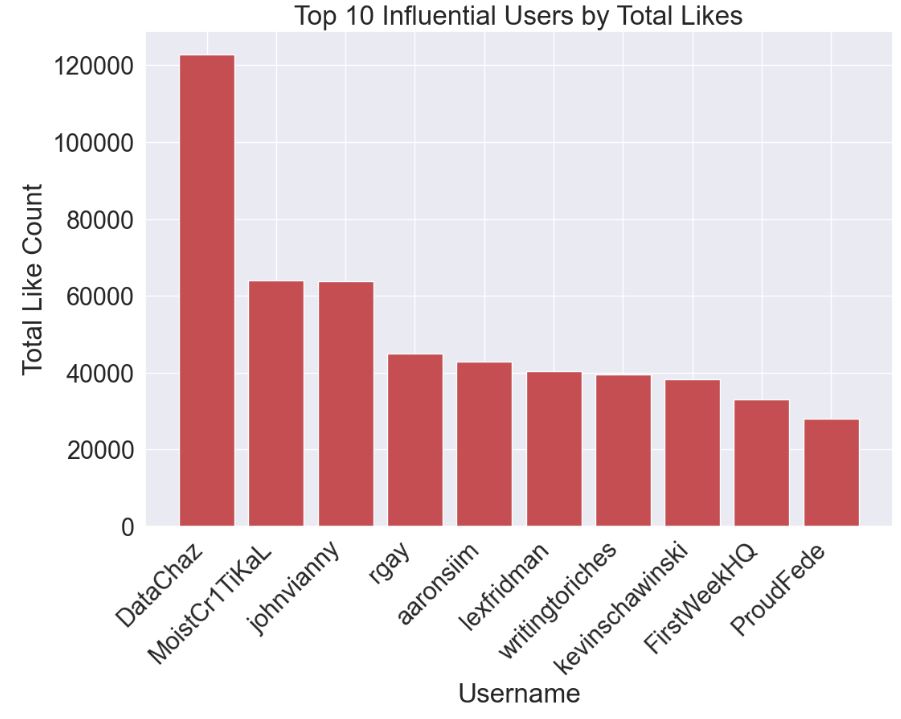
Let’s plot Top 10 Influential Users by Total Likes

user_likes = df.groupby(‘username’)[‘like_count’].sum().reset_index()
user_likes_sorted = user_likes.sort_values(by=’like_count’, ascending=False).head(10)

fig, ax = plt.subplots(figsize=(12, 8))
ax.bar(user_likes_sorted[‘username’], user_likes_sorted[‘like_count’], color=’r’)

plt.xlabel(‘Username’)
plt.ylabel(‘Total Like Count’)
plt.title(‘Top 10 Influential Users by Total Likes’)

plt.xticks(rotation=45, ha=’right’)

plt.show()

Stock Impact

Let’s compare stock impacts in Q1’23

start_date = ‘2023-01-04’
end_date = ‘2023-03-29’
ticker_symbols = [‘MSFT’, ‘GOOGL’, ‘AMZN’, ‘META’, ‘AAPL’,’TSLA’]
stocks_df = yf.download(ticker_symbols, start=start_date, end=end_date)[‘Adj Close’]

[*********************100%***********************]  6 of 6 completed

Number of tweets per day
tweets_by_day = df.groupby(pd.Grouper(key=’date’, freq=’D’)).size().reset_index()
tweets_by_day.columns = [‘date’, ‘count’]

import matplotlib.dates as mdates

fig, ax1 = plt.subplots(figsize=(20, 10))

ax1.bar(tweets_by_day[‘date’], tweets_by_day[‘count’], alpha=0.5)
ax1.set_xlabel(‘Date’)
ax1.set_ylabel(‘Tweet Count’)
ax1.tick_params(axis=’x’)
ax1.xaxis.set_major_formatter(mdates.DateFormatter(‘%Y-%m-%d’))

ax2 = ax1.twinx()
for symbol in ticker_symbols:
ax2.plot(stocks_df.index, stocks_df[symbol], label=symbol,linewidth=4)
ax2.set_ylabel(‘Stock Price’)
ax2.legend(loc=’upper left’)

plt.title(‘Stock Prices and Tweet Counts’)
plt.tight_layout()
plt.show()

Bigrams/Trigrams Counts

Let’s perform the Text Analysis using Top Bigrams and Trigrams.

We need the function to get n-grams

def get_top_n_ngrams(corpus, n=None, ngram=2):
vec = CountVectorizer(ngram_range=(ngram, ngram), stop_words=’english’).fit(corpus)
bag_of_words = vec.transform(corpus)
sum_words = bag_of_words.sum(axis=0)
words_freq = [(word, sum_words[0, idx]) for word, idx in vec.vocabulary_.items()]
words_freq = sorted(words_freq, key=lambda x: x[1], reverse=True)
return words_freq[:n]

Get top 10 bigrams
common_bigrams = get_top_n_ngrams(df[‘processed_content’], 10, ngram=2)

Get top 10 trigrams
common_trigrams = get_top_n_ngrams(df[‘processed_content’], 10, ngram=3)

and perform the data object conversion

df_bigrams = pd.DataFrame(common_bigrams, columns=[‘NgramText’, ‘count’])
df_trigrams = pd.DataFrame(common_trigrams, columns=[‘NgramText’, ‘count’])

Let’s plot the top 10 bigram count

plt.figure(figsize=(15, 6))
sns.barplot(data=df_bigrams[1:], x=’NgramText’, y=’count’, palette=’magma’)
plt.title(‘Bigram Counts’)
plt.xticks(rotation=45)
plt.show()

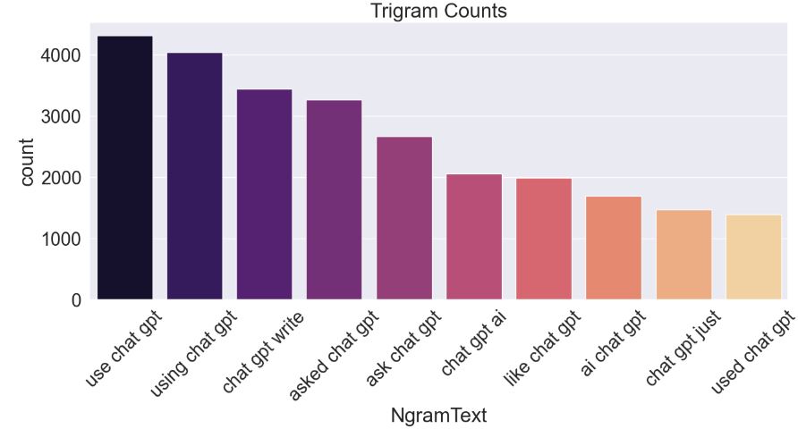
Let’s plot the top 10 trigram count

plt.figure(figsize=(15, 6))
sns.barplot(data=df_trigrams, x=’NgramText’, y=’count’, palette=’magma’)
plt.title(‘Trigram Counts’)
plt.xticks(rotation=45)
plt.show()

Let’s exclude ‘chat’, ‘gpt’, and ‘chatgpt’ from n-grams to get better results focusing on other aspects related to ChatGPT.

We need the modified function to exclude certain keywords from the ngrams
def get_top_n_ngrams(corpus, n=None, ngram=2, exclude_keywords=None):
if exclude_keywords is None:
exclude_keywords = []

vec = CountVectorizer(ngram_range=(ngram, ngram), stop_words='english').fit(corpus)
bag_of_words = vec.transform(corpus)
sum_words = bag_of_words.sum(axis=0) 
words_freq = [(word, sum_words[0, idx]) for word, idx in vec.vocabulary_.items()]
words_freq = sorted(words_freq, key=lambda x: x[1], reverse=True)

# Exclude n-grams containing specified keywords
words_freq = [item for item in words_freq if not any(keyword in item[0] for keyword in exclude_keywords)]

return words_freq[:n]

Let’s get top 10 bigrams
common_bigrams = get_top_n_ngrams(df[‘processed_content’], 10, ngram=2, exclude_keywords=[‘chat’, ‘gpt’, ‘chatgpt’])

Let’s get top 10 trigrams
common_trigrams = get_top_n_ngrams(df[‘processed_content’], 10, ngram=3, exclude_keywords=[‘chat’, ‘gpt’, ‘chatgpt’])

converting the lists to data frames
df_bigrams = pd.DataFrame(common_bigrams, columns=[‘NgramText’, ‘count’])
df_trigrams = pd.DataFrame(common_trigrams, columns=[‘NgramText’, ‘count’])

Modified Bigram Counts:

plt.figure(figsize=(15, 6))
sns.barplot(data=df_bigrams, x=’NgramText’, y=’count’, palette=’magma’)
plt.title(‘Bigram Counts’)
plt.xticks(rotation=45)
plt.show()

Modified Trigram Counts:

plt.figure(figsize=(15, 6))
sns.barplot(data=df_trigrams, x=’NgramText’, y=’count’, palette=’magma’)
plt.title(‘Trigram Counts’)
plt.xticks(rotation=45)
plt.show()

NLP Word Clouds

Initialize the lemmatizer:
wordnet_lem = WordNetLemmatizer()

Lemmatize processed text and join everything in a list:
df[‘content_lem’] = df[‘processed_content’].apply(wordnet_lem.lemmatize)
all_words_lem = ‘ ‘.join([word for word in df[‘content_lem’]])

Unigram Word Cloud:

from random import choice

def custom_color_func(word, font_size, position, orientation, random_state=None, **kwargs):
colors = [‘#1DA1F2’, ‘#00CC96’, ‘#FF5733’, ‘#FFC300’, ‘#E91E63’, ‘#9C27B0’, ‘#673AB7’]
return choice(colors)

stopwords = set(STOPWORDS)

wordcloud_twitter = WordCloud(height=2000, width=2000,
background_color=”white”,
stopwords=stopwords, color_func=custom_color_func).generate(all_words_lem)

plt.figure(figsize=[10, 10])
plt.axis(‘off’)
plt.tight_layout(pad=0)
plt.imshow(wordcloud_twitter.recolor(color_func=custom_color_func), interpolation=”bilinear”)

plt.savefig(“twitter_unigram.png”, format=”png”)

plt.show()

Mentions Word Cloud:

Extract mentions and concatenate all mentions in one string
all_mentions = ‘ ‘.join([mention[1:] for mentions in df[‘content’].str.findall(r’@\w+’) for mention in mentions])

Generate a word cloud image
wordcloud_twitter = WordCloud(height=2000, width=2000,
background_color=”white”,
stopwords=stopwords, color_func=custom_color_func).generate(all_mentions)

plt.figure(figsize=[10,10])
plt.axis(‘off’)
plt.tight_layout(pad=0)
plt.imshow(wordcloud_twitter.recolor(color_func=custom_color_func), interpolation=”bilinear”)

plt.savefig(“twitter_logo_unigram_mentions.png”, format=”png”)

plt.show()

Hashtag Word Cloud

Extract hashtags and concatenate all hashtags in one string
all_hashtags = ‘ ‘.join([hashtag[1:] for hashtags in df[‘content’].str.findall(r’#\w+’) for hashtag in hashtags])

Generate a word cloud image
wordcloud_twitter = WordCloud(height=2000, width=2000,
background_color=”white”,
stopwords=stopwords, color_func=custom_color_func).generate(all_hashtags)

plt.figure(figsize=[10,10])
plt.axis(‘off’)
plt.tight_layout(pad=0)
plt.imshow(wordcloud_twitter.recolor(color_func=custom_color_func), interpolation=”bilinear”)

plt.savefig(“twitter_logo_unigram_hashtags.png”, format=”png”)

plt.show()

Conclusions

• Max number of ChatGPT-related tweets per week is > 50k (2023-03-13).
• Ben_Ccarter is the most active user in terms of the tweet volume.
• DataChaz is the most influential user in terms of total likes.
• MSFT and META stock prices in Q1’23 were most sensitive to the ChatGPT content on Twitter.
• “Language model” and “search engine” are among top 10 bigram counts.
• “Large language model”, “15 min chart”, and “trades 15 min” are among top 10 trigram counts.
• We have generated and compared the Unigram, Mentions, and Hashtag NLP Word Clouds.

Explore More

• Trending YouTube Video Data Science, NLP Predictions & Sentiment Analysis
• AI-Guided Drug Recommendation
• Semantic Analysis and NLP Visualizations of Wine Reviews
• Drug Review Data Analytics

References

• Cracking the ChatGPT Code: A Deep Dive into 500,000 Tweets using Advanced NLP Techniques

• Comprehensive Analysis of 500K Tweets on ChatGPT
• Effortlessly Scraping Massive Twitter Data with snscrape: A Guide to Scraping 1000,000 Tweets in Less than a Day
• Comprehensive Analysis of 500K Tweets on ChatGPT.ipynb
• How to Build a Sentiment Analysis Application with ChatGPT and Druid

Embed Socials

• Advanced NLP Analysis & Stock Impact of ChatGPT-Related Tweets Q1’23