Comparison of 20 ML + NLP Algorithms for SMS Spam-Ham Binary Classification

Photo by Hannes Johnson on Unsplash

• The goal of this post is to find the best NLP Spam-Ham binary classifier using the public-domain SMS text message dataset.

• Considering various modes of communication, SMS messages are the most popular means for both informal and formal conversations. 
• This showcase mainly deals with the comparative analysis of detecting Spam SMS texts by various supervised ML scikit-learn classification algorithms.
• We will consider various evaluation metrics and scoring for quantifying the quality of model predictions.

The Python workflow consists of the following 5 steps:

1. Importing key libraries and downloading input data
2. Exploratory Data Analysis (EDA)
3. NLP Processing
4. Supervised ML Binary Classification
5. Model Performance QC Analysis

Read more here.

Data Preparation

Let’s set the working directory SPAM

import os
os.chdir(‘./SPAM’)
os. getcwd()

and import the following libraries

import pandas as pd
import numpy as np
import matplotlib.pyplot as plt
import seaborn as sns
sns.set()

import re
import string
from wordcloud import WordCloud
from collections import Counter

import warnings
warnings.filterwarnings(‘ignore’)

from nltk import sent_tokenize, word_tokenize
from nltk.corpus import stopwords
from nltk.stem import PorterStemmer

from sklearn.feature_extraction.text import TfidfVectorizer
from sklearn.model_selection import train_test_split
from sklearn.naive_bayes import MultinomialNB
from sklearn.ensemble import RandomForestClassifier

from sklearn.metrics import accuracy_score, precision_score, recall_score, f1_score

from scikitplot.metrics import plot_confusion_matrix, plot_roc

Let’s import the input dataset

data = pd.read_csv(‘SPAM text message 20170820 – Data.csv’)
data.head()

print(data.shape)

(5572, 2)

data.isnull().sum()

Category    0
Message     0
dtype: int64

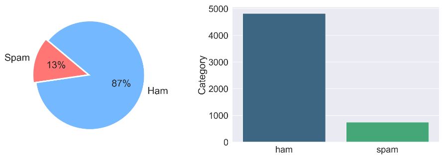
data[‘Category’].value_counts()

ham     4825
spam     747
Name: Category, dtype: int64

Let’s plot Category

labels = [‘Spam’, ‘Ham’]
sizes = [747, 4825]
custom_colours = [‘#ff7675’, ‘#74b9ff’]

sns.set(font_scale=2)

plt.figure(figsize=(20, 6), dpi=227)
plt.subplot(1, 2, 1)
plt.pie(sizes, labels = labels, textprops={‘fontsize’: 24}, startangle=140,
autopct=’%1.0f%%’, colors=custom_colours, explode=[0, 0.05])

plt.subplot(1, 2, 2)
sns.barplot(x = data[‘Category’].unique(), y = data[‘Category’].value_counts(), palette= ‘viridis’)

plt.show()

Exploratory Data Analysis (EDA)

Let’s count total words vs total characters

data[‘Total Words’] = data[‘Message’].apply(lambda x: len(x.split()))

def count_total_words(text):
char = 0
for word in text.split():
char += len(word)
return char

data[‘Total Chars’] = data[“Message”].apply(count_total_words)
#data.head()

plt.figure(figsize = (10, 6))
sns.set(font_scale=2)
sns.kdeplot(x = data[‘Total Words’], hue= data[‘Category’], palette= ‘winter’, shade = True)
plt.show()

plt.figure(figsize = (10, 6))
sns.set(font_scale=2)
sns.kdeplot(x = data[‘Total Chars’], hue= data[‘Category’], palette= ‘winter’, shade = True)
plt.show()

NLP Processing

Let’s implement the following text processing steps: Lowercasing, Removing URLs, Removing Punctuations, Removing stopwords, and Stemming.

def convert_lowercase(text):
text = text.lower()
return text

data[‘Message’] = data[‘Message’].apply(convert_lowercase)
def remove_url(text):
re_url = re.compile(‘https?://\S+|www.\S+’)
return re_url.sub(”, text)

data[‘Message’] = data[‘Message’].apply(remove_url)
exclude = string.punctuation

def remove_punc(text):
return text.translate(str.maketrans(”, ”, exclude))

data[‘Message’] = data[‘Message’].apply(remove_punc)
def remove_stopwords(text):
new_list = []
words = word_tokenize(text)
stopwrds = stopwords.words(‘english’)
for word in words:
if word not in stopwrds:
new_list.append(word)
return ‘ ‘.join(new_list)

data[‘Message’] = data[‘Message’].apply(remove_stopwords)
def perform_stemming(text):
stemmer = PorterStemmer()
new_list = []
words = word_tokenize(text)
for word in words:
new_list.append(stemmer.stem(word))

return " ".join(new_list)

data[‘Message’] = data[‘Message’].apply(perform_stemming)
data[‘Total Words After Transformation’] = data[‘Message’].apply(lambda x: np.log(len(x.split())))
#data.head()

Data Visualization

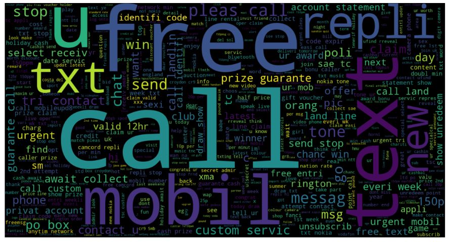
Let’s plot the following two word clouds

text = ” “.join(data[data[‘Category’] == ‘spam’][‘Message’])
plt.figure(figsize = (15, 10))
wordcloud = WordCloud(max_words=500, height= 800, width = 1500, background_color=”black”, colormap= ‘viridis’).generate(text)
plt.imshow(wordcloud, interpolation=”bilinear”)
plt.axis(‘off’)
plt.show()

SPAM WORD CLOUD:

HAM WORD CLOUD:

text = ” “.join(data[data[‘Category’] == ‘ham’][‘Message’])
plt.figure(figsize = (15, 10))
wordcloud = WordCloud(max_words=500, height= 800, width = 1500, background_color=”black”, colormap= ‘viridis’).generate(text)
plt.imshow(wordcloud, interpolation=”bilinear”)
plt.axis(‘off’)
plt.show()

Supervised ML Binary Classification

Let’s prepare the data for ML model training – target/features/train/test data splitting and applying TfidfVectorizer

X = data[“Message”]
y = data[‘Category’].values

X_train, X_test, y_train, y_test = train_test_split(X, y, test_size= 0.2, random_state= 42, stratify = y)

tfidf = TfidfVectorizer(max_features= 2500, min_df= 2)
X_train = tfidf.fit_transform(X_train).toarray()
X_test = tfidf.transform(X_test).toarray()

Let’s introduce the function train_model

from sklearn.metrics import cohen_kappa_score,matthews_corrcoef,jaccard_score
from sklearn.metrics import classification_report
target_names = [‘Spam’, ‘Ham’]
def train_model(model):
model.fit(X_train, y_train)
y_pred = model.predict(X_test)
y_prob = model.predict_proba(X_test)
accuracy = round(accuracy_score(y_test, y_pred), 3)
precision = round(precision_score(y_test, y_pred), 3)
recall = round(recall_score(y_test, y_pred), 3)
f1 = round(f1_score(y_test, y_pred), 3)
cohen = round(cohen_kappa_score(y_test, y_pred), 3)
matthews = round(matthews_corrcoef(y_test, y_pred), 3)
jaccard = round(matthews_corrcoef(y_test, y_pred), 3)
print(f’Accuracy of the model: {accuracy}’)
print(f’Precision Score of the model: {precision}’)
print(f’Recall Score of the model: {recall}’)
print(f’F1-Score of the model: {f1}’)
print(f’Cohen-Score of the model: {cohen}’)
print(f’matthews_corrcoef of the model: {matthews}’)
#print(f’Jaccard-Score of the model: {jaccard}’)
print(classification_report(y_test, y_pred, target_names=target_names))

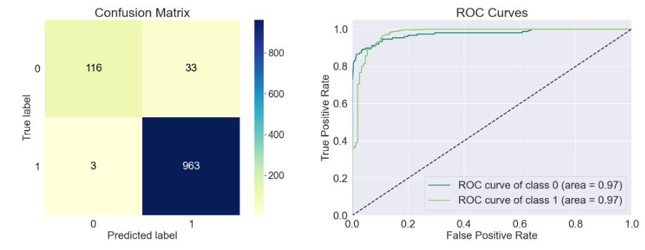
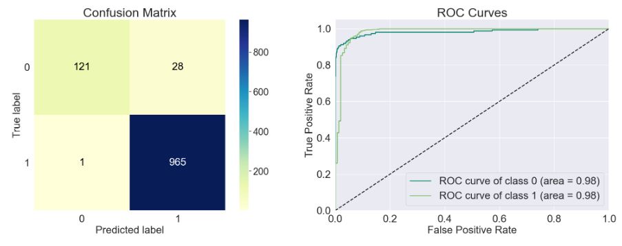
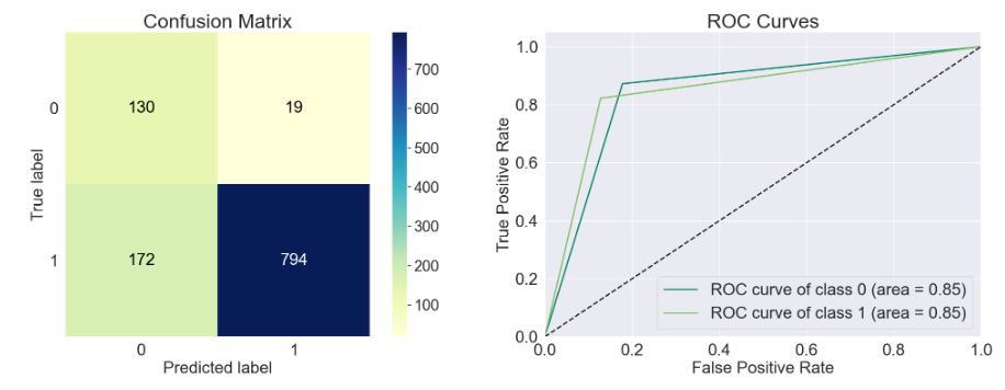
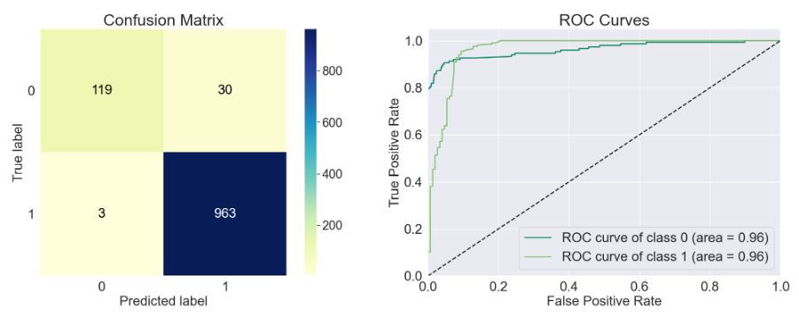
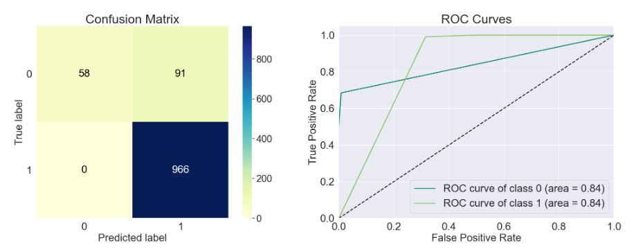
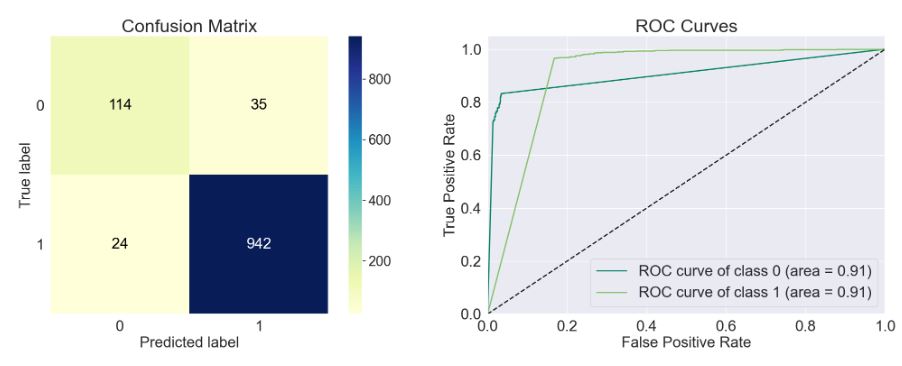
sns.set_context('notebook', font_scale= 2)
fig, ax = plt.subplots(1, 2, figsize = (25,  8))
ax1 = plot_confusion_matrix(y_test, y_pred, ax= ax[0], cmap= 'YlGnBu')
ax2 = plot_roc(y_test, y_prob, ax= ax[1], plot_macro= False, plot_micro= False, cmap= 'summer')

Let’s proceed with model training for various classifiers:

from sklearn.base import ClassifierMixin
from sklearn.utils import all_estimators
classifiers=[est for est in all_estimators() if issubclass(est[1], ClassifierMixin)]
print(classifiers)

[('AdaBoostClassifier', <class 'sklearn.ensemble._weight_boosting.AdaBoostClassifier'>), ('BaggingClassifier', <class 'sklearn.ensemble._bagging.BaggingClassifier'>), ('BernoulliNB', <class 'sklearn.naive_bayes.BernoulliNB'>), ('CalibratedClassifierCV', <class 'sklearn.calibration.CalibratedClassifierCV'>), ('CategoricalNB', <class 'sklearn.naive_bayes.CategoricalNB'>), ('ClassifierChain', <class 'sklearn.multioutput.ClassifierChain'>), ('ComplementNB', <class 'sklearn.naive_bayes.ComplementNB'>), ('DecisionTreeClassifier', <class 'sklearn.tree._classes.DecisionTreeClassifier'>), ('DummyClassifier', <class 'sklearn.dummy.DummyClassifier'>), ('ExtraTreeClassifier', <class 'sklearn.tree._classes.ExtraTreeClassifier'>), ('ExtraTreesClassifier', <class 'sklearn.ensemble._forest.ExtraTreesClassifier'>), ('GaussianNB', <class 'sklearn.naive_bayes.GaussianNB'>), ('GaussianProcessClassifier', <class 'sklearn.gaussian_process._gpc.GaussianProcessClassifier'>), ('GradientBoostingClassifier', <class 'sklearn.ensemble._gb.GradientBoostingClassifier'>), ('HistGradientBoostingClassifier', <class 'sklearn.ensemble._hist_gradient_boosting.gradient_boosting.HistGradientBoostingClassifier'>), ('KNeighborsClassifier', <class 'sklearn.neighbors._classification.KNeighborsClassifier'>), ('LabelPropagation', <class 'sklearn.semi_supervised._label_propagation.LabelPropagation'>), ('LabelSpreading', <class 'sklearn.semi_supervised._label_propagation.LabelSpreading'>), ('LinearDiscriminantAnalysis', <class 'sklearn.discriminant_analysis.LinearDiscriminantAnalysis'>), ('LinearSVC', <class 'sklearn.svm._classes.LinearSVC'>), ('LogisticRegression', <class 'sklearn.linear_model._logistic.LogisticRegression'>), ('LogisticRegressionCV', <class 'sklearn.linear_model._logistic.LogisticRegressionCV'>), ('MLPClassifier', <class 'sklearn.neural_network._multilayer_perceptron.MLPClassifier'>), ('MultiOutputClassifier', <class 'sklearn.multioutput.MultiOutputClassifier'>), ('MultinomialNB', <class 'sklearn.naive_bayes.MultinomialNB'>), ('NearestCentroid', <class 'sklearn.neighbors._nearest_centroid.NearestCentroid'>), ('NuSVC', <class 'sklearn.svm._classes.NuSVC'>), ('OneVsOneClassifier', <class 'sklearn.multiclass.OneVsOneClassifier'>), ('OneVsRestClassifier', <class 'sklearn.multiclass.OneVsRestClassifier'>), ('OutputCodeClassifier', <class 'sklearn.multiclass.OutputCodeClassifier'>), ('PassiveAggressiveClassifier', <class 'sklearn.linear_model._passive_aggressive.PassiveAggressiveClassifier'>), ('Perceptron', <class 'sklearn.linear_model._perceptron.Perceptron'>), ('QuadraticDiscriminantAnalysis', <class 'sklearn.discriminant_analysis.QuadraticDiscriminantAnalysis'>), ('RadiusNeighborsClassifier', <class 'sklearn.neighbors._classification.RadiusNeighborsClassifier'>), ('RandomForestClassifier', <class 'sklearn.ensemble._forest.RandomForestClassifier'>), ('RidgeClassifier', <class 'sklearn.linear_model._ridge.RidgeClassifier'>), ('RidgeClassifierCV', <class 'sklearn.linear_model._ridge.RidgeClassifierCV'>), ('SGDClassifier', <class 'sklearn.linear_model._stochastic_gradient.SGDClassifier'>), ('SVC', <class 'sklearn.svm._classes.SVC'>), ('StackingClassifier', <class 'sklearn.ensemble._stacking.StackingClassifier'>), ('VotingClassifier', <class 'sklearn.ensemble._voting.VotingClassifier'>)]

• nb = MultinomialNB()
  train_model(nb)

Accuracy of the model: 0.968
Precision Score of the model: 0.967
Recall Score of the model: 0.997
F1-Score of the model: 0.982
Cohen-Score of the model: 0.848
matthews_corrcoef of the model: 0.855
              precision    recall  f1-score   support

        Spam       0.97      0.78      0.87       149
         Ham       0.97      1.00      0.98       966

    accuracy                           0.97      1115
   macro avg       0.97      0.89      0.92      1115
weighted avg       0.97      0.97      0.97      1115

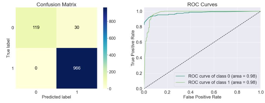
• rf = RandomForestClassifier(n_estimators= 300)
  train_model(rf)

Accuracy of the model: 0.973
Precision Score of the model: 0.97
Recall Score of the model: 1.0
F1-Score of the model: 0.985
Cohen-Score of the model: 0.873
matthews_corrcoef of the model: 0.88
              precision    recall  f1-score   support

        Spam       1.00      0.80      0.89       149
         Ham       0.97      1.00      0.98       966

    accuracy                           0.97      1115
   macro avg       0.98      0.90      0.94      1115
weighted avg       0.97      0.97      0.97      1115

• import sklearn
  ada = sklearn.ensemble._weight_boosting.AdaBoostClassifier()
  train_model(ada)

Accuracy of the model: 0.955
Precision Score of the model: 0.962
Recall Score of the model: 0.988
F1-Score of the model: 0.974
Cohen-Score of the model: 0.791
matthews_corrcoef of the model: 0.796
              precision    recall  f1-score   support

        Spam       0.90      0.74      0.82       149
         Ham       0.96      0.99      0.97       966

    accuracy                           0.96      1115
   macro avg       0.93      0.87      0.90      1115
weighted avg       0.95      0.96      0.95      1115

• model=sklearn.naive_bayes.BernoulliNB()
  train_model(model)

Accuracy of the model: 0.974
Precision Score of the model: 0.972
Recall Score of the model: 0.999
F1-Score of the model: 0.985
Cohen-Score of the model: 0.878
matthews_corrcoef of the model: 0.884
              precision    recall  f1-score   support

        Spam       0.99      0.81      0.89       149
         Ham       0.97      1.00      0.99       966

    accuracy                           0.97      1115
   macro avg       0.98      0.91      0.94      1115
weighted avg       0.97      0.97      0.97      1115

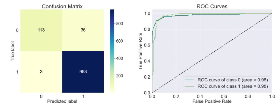
• model=sklearn.calibration.CalibratedClassifierCV()
  train_model(model)

Accuracy of the model: 0.978
Precision Score of the model: 0.98
Recall Score of the model: 0.995
F1-Score of the model: 0.987
Cohen-Score of the model: 0.899
matthews_corrcoef of the model: 0.901
              precision    recall  f1-score   support

        Spam       0.96      0.87      0.91       149
         Ham       0.98      0.99      0.99       966

    accuracy                           0.98      1115
   macro avg       0.97      0.93      0.95      1115
weighted avg       0.98      0.98      0.98      1115

• model=sklearn.tree._classes.DecisionTreeClassifier()
  train_model(model)

Accuracy of the model: 0.952
Precision Score of the model: 0.97
Recall Score of the model: 0.975
F1-Score of the model: 0.973
Cohen-Score of the model: 0.792
matthews_corrcoef of the model: 0.792
              precision    recall  f1-score   support

        Spam       0.83      0.81      0.82       149
         Ham       0.97      0.98      0.97       966

    accuracy                           0.95      1115
   macro avg       0.90      0.89      0.90      1115
weighted avg       0.95      0.95      0.95      1115

• model=sklearn.tree._classes.ExtraTreeClassifier()
  train_model(model)

Accuracy of the model: 0.952
Precision Score of the model: 0.972
Recall Score of the model: 0.973
F1-Score of the model: 0.973
Cohen-Score of the model: 0.794
matthews_corrcoef of the model: 0.794
              precision    recall  f1-score   support

        Spam       0.82      0.82      0.82       149
         Ham       0.97      0.97      0.97       966

    accuracy                           0.95      1115
   macro avg       0.90      0.90      0.90      1115
weighted avg       0.95      0.95      0.95      1115

• model=sklearn.naive_bayes.GaussianNB()
  train_model(model)

Accuracy of the model: 0.829
Precision Score of the model: 0.977
Recall Score of the model: 0.822
F1-Score of the model: 0.893
Cohen-Score of the model: 0.484
matthews_corrcoef of the model: 0.532
              precision    recall  f1-score   support

        Spam       0.43      0.87      0.58       149
         Ham       0.98      0.82      0.89       966

    accuracy                           0.83      1115
   macro avg       0.70      0.85      0.73      1115
weighted avg       0.90      0.83      0.85      1115

• model=sklearn.gaussian_process._gpc.GaussianProcessClassifier()
  train_model(model)

Accuracy of the model: 0.948
Precision Score of the model: 0.943
Recall Score of the model: 1.0
F1-Score of the model: 0.971
Cohen-Score of the model: 0.731
matthews_corrcoef of the model: 0.759
              precision    recall  f1-score   support

        Spam       1.00      0.61      0.76       149
         Ham       0.94      1.00      0.97       966

    accuracy                           0.95      1115
   macro avg       0.97      0.81      0.86      1115
weighted avg       0.95      0.95      0.94      1115

• model=sklearn.ensemble._gb.GradientBoostingClassifier()
  train_model(model)

Accuracy of the model: 0.961
Precision Score of the model: 0.957
Recall Score of the model: 1.0
F1-Score of the model: 0.978
Cohen-Score of the model: 0.81
matthews_corrcoef of the model: 0.825
              precision    recall  f1-score   support

        Spam       1.00      0.71      0.83       149
         Ham       0.96      1.00      0.98       966

    accuracy                           0.96      1115
   macro avg       0.98      0.86      0.90      1115
weighted avg       0.96      0.96      0.96      1115

• model=sklearn.ensemble._hist_gradient_boosting.gradient_boosting.HistGradientBoostingClassifier()
  train_model(model)

Accuracy of the model: 0.97
Precision Score of the model: 0.97
Recall Score of the model: 0.997
F1-Score of the model: 0.983
Cohen-Score of the model: 0.862
matthews_corrcoef of the model: 0.867
              precision    recall  f1-score   support

        Spam       0.98      0.80      0.88       149
         Ham       0.97      1.00      0.98       966

    accuracy                           0.97      1115
   macro avg       0.97      0.90      0.93      1115
weighted avg       0.97      0.97      0.97      1115

• model=sklearn.neighbors._classification.KNeighborsClassifier()
  train_model(model)

Accuracy of the model: 0.918
Precision Score of the model: 0.914
Recall Score of the model: 1.0
F1-Score of the model: 0.955
Cohen-Score of the model: 0.525
matthews_corrcoef of the model: 0.596
              precision    recall  f1-score   support

        Spam       1.00      0.39      0.56       149
         Ham       0.91      1.00      0.96       966

    accuracy                           0.92      1115
   macro avg       0.96      0.69      0.76      1115
weighted avg       0.93      0.92      0.90      1115

• model=sklearn.semi_supervised._label_propagation.LabelPropagation()
  train_model(model)

Accuracy of the model: 0.951
Precision Score of the model: 0.946
Recall Score of the model: 1.0
F1-Score of the model: 0.972
Cohen-Score of the model: 0.748
matthews_corrcoef of the model: 0.773
              precision    recall  f1-score   support

        Spam       1.00      0.63      0.77       149
         Ham       0.95      1.00      0.97       966

    accuracy                           0.95      1115
   macro avg       0.97      0.82      0.87      1115
weighted avg       0.95      0.95      0.95      1115

• model=sklearn.discriminant_analysis.LinearDiscriminantAnalysis()
  train_model(model)

Accuracy of the model: 0.947
Precision Score of the model: 0.964
Recall Score of the model: 0.975
F1-Score of the model: 0.97
Cohen-Score of the model: 0.764
matthews_corrcoef of the model: 0.765
              precision    recall  f1-score   support

        Spam       0.83      0.77      0.79       149
         Ham       0.96      0.98      0.97       966

    accuracy                           0.95      1115
   macro avg       0.90      0.87      0.88      1115
weighted avg       0.95      0.95      0.95      1115

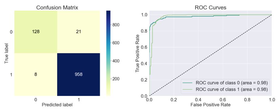
• LinearSVC_classifier = sklearn.svm._classes.SVC(kernel=’linear’,probability=True)
  model=LinearSVC_classifier
  train_model(model)

Accuracy of the model: 0.976
Precision Score of the model: 0.976
Recall Score of the model: 0.997
F1-Score of the model: 0.986
Cohen-Score of the model: 0.889
matthews_corrcoef of the model: 0.892
              precision    recall  f1-score   support

        Spam       0.98      0.84      0.90       149
         Ham       0.98      1.00      0.99       966

    accuracy                           0.98      1115
   macro avg       0.98      0.92      0.94      1115
weighted avg       0.98      0.98      0.97      1115

model=sklearn.linear_model._logistic.LogisticRegression()
train_model(model)

Accuracy of the model: 0.965
Precision Score of the model: 0.964
Recall Score of the model: 0.997
F1-Score of the model: 0.98
Cohen-Score of the model: 0.833
matthews_corrcoef of the model: 0.842
              precision    recall  f1-score   support

        Spam       0.97      0.76      0.85       149
         Ham       0.96      1.00      0.98       966

    accuracy                           0.97      1115
   macro avg       0.97      0.88      0.92      1115
weighted avg       0.97      0.97      0.96      1115

• model=sklearn.linear_model._logistic.LogisticRegressionCV()
  train_model(model)

Accuracy of the model: 0.974
Precision Score of the model: 0.979
Recall Score of the model: 0.992
F1-Score of the model: 0.985
Cohen-Score of the model: 0.883
matthews_corrcoef of the model: 0.885
              precision    recall  f1-score   support

        Spam       0.94      0.86      0.90       149
         Ham       0.98      0.99      0.99       966

    accuracy                           0.97      1115
   macro avg       0.96      0.93      0.94      1115
weighted avg       0.97      0.97      0.97      1115

• model=sklearn.neural_network._multilayer_perceptron.MLPClassifier()
  train_model(model)

Accuracy of the model: 0.975
Precision Score of the model: 0.98
Recall Score of the model: 0.992
F1-Score of the model: 0.986
Cohen-Score of the model: 0.888
matthews_corrcoef of the model: 0.889
              precision    recall  f1-score   support

        Spam       0.94      0.87      0.90       149
         Ham       0.98      0.99      0.99       966

    accuracy                           0.97      1115
   macro avg       0.96      0.93      0.94      1115
weighted avg       0.97      0.97      0.97      1115

• model=sklearn.discriminant_analysis.QuadraticDiscriminantAnalysis()
  train_model(model)

Accuracy of the model: 0.944
Precision Score of the model: 0.955
Recall Score of the model: 0.982
F1-Score of the model: 0.968
Cohen-Score of the model: 0.739
matthews_corrcoef of the model: 0.744
              precision    recall  f1-score   support

        Spam       0.86      0.70      0.77       149
         Ham       0.95      0.98      0.97       966

    accuracy                           0.94      1115
   macro avg       0.91      0.84      0.87      1115
weighted avg       0.94      0.94      0.94      1115

• model=sklearn.svm._classes.SVC(probability=True)
  train_model(model)

Accuracy of the model: 0.971
Precision Score of the model: 0.971
Recall Score of the model: 0.997
F1-Score of the model: 0.984
Cohen-Score of the model: 0.866
matthews_corrcoef of the model: 0.871
              precision    recall  f1-score   support

        Spam       0.98      0.81      0.88       149
         Ham       0.97      1.00      0.98       966

    accuracy                           0.97      1115
   macro avg       0.97      0.90      0.93      1115
weighted avg       0.97      0.97      0.97      1115

Summary

• This study draws the contrast on strengths, drawbacks, and limitations of some of the existing classifiers that use the approaches of supervised ML to detect spam text messages in real time.
• The open-source Kaggle dataset consists of 5572 SMS messages collected for training on different ML algorithms. The proportion of the minority class “Spam” is 13.4% of the entire dataset (moderate degree of imbalance).

• As a key takeaway, let’s look at the bar plot of top 8 best performing ML algorithms in terms of the F1-score (> 0.8)

plt.figure(figsize=(14,6))

x = [‘SVC’, ‘MLP’, ‘LRCV’,’HGBC’,’DTC’,’RFC’,’CCCV’,’BNB’]
y = [0.88, 0.90, 0.9,0.88,0.82,0.89,0.91,0.89]
plt.title(‘F1-Score Spam’, fontsize=24)
plt.bar(x,y)
plt.show()

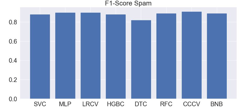
The worst performing ML algorithms in terms of the F1-score (< 0.7) are GaussianNB and KNN.

• We have compared various evaluation metrics and scoring for quantifying the quality of ML predictions: accuracy, precision, recall, F1-score, Cohen’s kappa, and matthews_corrcoef. We have also plotted the confusion matrix and the ROC curves.
• The study confirms that the F1-score is the best metric to use for classification models as it provides robust results for both balanced and imbalanced datasets, unlike accuracy or ROC curves.

• Results show that MLP, Logistic Regression CV, Linear SVC, and Calibrated Classifier CV yield ~90% F1-score, and so they outperform other ML algorithms in the detection of spam content.

• Bottom Line: Regardless of the nature of spam content, it can still be detected and deleted automatically.

Explore More

• Improved Multiple-Model ML/DL Credit Card Fraud Detection: F1=88% & ROC=91%
• Data-Driven ML Credit Card Fraud Detection