
- Globally, cardiovascular disease (CVD) is the primary cause of morbidity and mortality, accounting for more than 70% of all fatalities.
- Machine learning (ML) can be used to predict the risk of a heart attack. The algorithms used for this task would be supervised ML algorithms, such as Random Forest, Logistic Regression, Support Vector Machines, etc. These algorithms can be trained on data from past heart attack patients and then used to predict the likelihood of a heart attack in a new patient. The features used for this prediction could include age, gender, lifestyle factors, medical history, and other relevant factors.
- In addition, technologies such as electrocardiograms (ECG) are also important for diagnosing CVD. However, popular classification models based on supervised ML often fail to detect abnormal ECG effectively. Following recent research studies, we propose an ECG anomaly detection framework based on deep learning autoencoders.
- Autoencoders are a type of Artificial Neural Network (ANN) that is used to learn complex data representations and compress data effectively. Autoencoders are trained to learn a representation of the input data that has a lower dimensionality than the original input. This is done by learning to reconstruct the input data from a compressed representation. Autoencoders can be used for a variety of tasks, such as dimensionality reduction, denoising, and feature extraction.
- This post consists of the following two parts: (1) ECG Anomaly Detection using Autoencoders and (2) early heart attack detection using available supervised ML algorithms.
- About Input Kaggle Datasets:
- The first dataset contains the ECG readings of patients
- The second dataset is for heart attack classification using the following features
- Age : Age of the patient
- Sex : Sex of the patient
- exang: exercise induced angina (1 = yes; 0 = no)
- ca: number of major vessels (0-3)
- cp : Chest Pain type chest pain type
- Value 1: typical angina
- Value 2: atypical angina
- Value 3: non-anginal pain
- Value 4: asymptomatic
- trtbps : resting blood pressure (in mm Hg)
- chol : cholesterol in mg/dl fetched via BMI sensor
- fbs : (fasting blood sugar > 120 mg/dl) (1 = true; 0 = false)
- rest_ecg : resting electrocardiographic results
- Value 0: normal
- Value 1: having ST-T wave abnormality (T wave inversions and/or ST elevation or depression of > 0.05 mV)
- Value 2: showing probable or definite left ventricular hypertrophy by Estes’ criteria
- thalach : maximum heart rate achieved
- target : 0= less chance of heart attack 1= more chance of heart attack
Table of Contents
- ECG Autoencoder
- Input Dataset
- Exploratory Data Analysis (EDA)
- Feature Correlations
- Multiple ML/AI Models
- Feature Importance
- Model Performance
- Summary
- Explore More
Embed Socials:
ECG Autoencoder
Let’s set the working directory YOURPATH
import os
os.chdir(‘YOURPATH’)
os. getcwd()
and import the following libraries
import tensorflow as tf
import matplotlib.pyplot as plt
import numpy as np
import pandas as pd
from tensorflow.keras import layers, losses
from sklearn.model_selection import train_test_split
from tensorflow.keras.models import Model
Let’s read the input dataset
df = pd.read_csv(‘ecg.csv’, header=None)
Let’s perform the following data manipulations:
- Split data and labels
data = df.iloc[:,:-1].values
labels = df.iloc[:,-1].values
2. Split train and test data with test_size = 0.2
train_data, test_data, train_labels, test_labels = train_test_split(data, labels, test_size = 0.2, random_state = 21)
3. Normalization
min = tf.reduce_min(train_data)
max = tf.reduce_max(train_data)
train_data = (train_data – min)/(max – min)
test_data = (test_data – min)/(max – min)
4. Data format conversion
train_data = tf.cast(train_data, dtype=tf.float32)
test_data = tf.cast(test_data, dtype=tf.float32)
5. Label format conversion
train_labels = train_labels.astype(bool)
test_labels = test_labels.astype(bool)
6. Separate normal and abnormal ECG data
- Normal ECG data
n_train_data = train_data[train_labels]
n_test_data = test_data[test_labels] - Abnormal ECG data
- an_train_data = train_data[~train_labels]
- an_test_data = test_data[~test_labels]
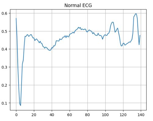
Lets plot a normal ECG
plt.plot(np.arange(140), n_train_data[0])
plt.grid()
plt.title(‘Normal ECG’)
plt.show()
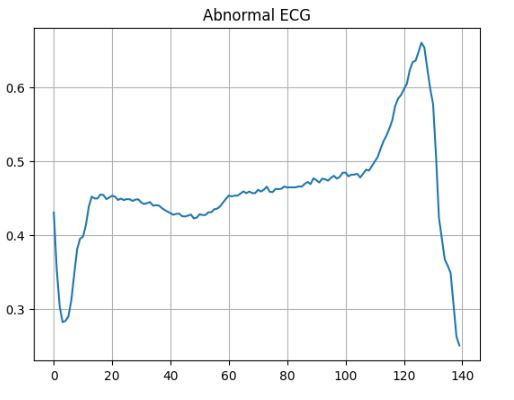
Lets plot an abnormal ECG
plt.plot(np.arange(140), an_train_data[0])
plt.grid()
plt.title(‘Abnormal ECG’)
plt.show()
Let’s introduce the detector = encoder + decoder class
class detector(Model):
def init(self):
super(detector, self).init()
self.encoder = tf.keras.Sequential([
layers.Dense(32, activation=’relu’),
layers.Dense(16, activation=’relu’),
layers.Dense(8, activation=’relu’)
])
self.decoder = tf.keras.Sequential([
layers.Dense(16, activation=’relu’),
layers.Dense(32, activation=’relu’),
layers.Dense(140, activation=’sigmoid’)
])
def call(self, x):
encoded = self.encoder(x)
decoded = self.decoder(encoded)
return decoded
Let’s compile and train the model
autoencoder = detector()
autoencoder.compile(optimizer=’adam’, loss=’mae’)
autoencoder.fit(n_train_data, n_train_data, epochs = 20, batch_size=512, validation_data=(n_test_data, n_test_data))
Epoch 1/20
5/5 [==============================] - 1s 42ms/step - loss: 0.0595 - val_loss: 0.0573
Epoch 2/20
5/5 [==============================] - 0s 7ms/step - loss: 0.0568 - val_loss: 0.0557
Epoch 3/20
5/5 [==============================] - 0s 8ms/step - loss: 0.0551 - val_loss: 0.0537
Epoch 4/20
5/5 [==============================] - 0s 7ms/step - loss: 0.0528 - val_loss: 0.0508
Epoch 5/20
5/5 [==============================] - 0s 7ms/step - loss: 0.0495 - val_loss: 0.0471
Epoch 6/20
5/5 [==============================] - 0s 7ms/step - loss: 0.0460 - val_loss: 0.0438
Epoch 7/20
5/5 [==============================] - 0s 7ms/step - loss: 0.0427 - val_loss: 0.0405
Epoch 8/20
5/5 [==============================] - 0s 7ms/step - loss: 0.0395 - val_loss: 0.0374
Epoch 9/20
5/5 [==============================] - 0s 7ms/step - loss: 0.0367 - val_loss: 0.0348
Epoch 10/20
5/5 [==============================] - 0s 7ms/step - loss: 0.0342 - val_loss: 0.0326
Epoch 11/20
5/5 [==============================] - 0s 7ms/step - loss: 0.0321 - val_loss: 0.0307
Epoch 12/20
5/5 [==============================] - 0s 7ms/step - loss: 0.0303 - val_loss: 0.0290
Epoch 13/20
5/5 [==============================] - 0s 7ms/step - loss: 0.0286 - val_loss: 0.0274
Epoch 14/20
5/5 [==============================] - 0s 8ms/step - loss: 0.0272 - val_loss: 0.0261
Epoch 15/20
5/5 [==============================] - 0s 7ms/step - loss: 0.0261 - val_loss: 0.0253
Epoch 16/20
5/5 [==============================] - 0s 8ms/step - loss: 0.0253 - val_loss: 0.0247
Epoch 17/20
5/5 [==============================] - 0s 7ms/step - loss: 0.0247 - val_loss: 0.0241
Epoch 18/20
5/5 [==============================] - 0s 7ms/step - loss: 0.0241 - val_loss: 0.0234
Epoch 19/20
5/5 [==============================] - 0s 7ms/step - loss: 0.0235 - val_loss: 0.0228
Epoch 20/20
5/5 [==============================] - 0s 8ms/step - loss: 0.0228 - val_loss: 0.0222
Let’s define a function in order to plot the original ECG and reconstructed ones and also show the error
def plot(data, n):
enc_img = autoencoder.encoder(data)
dec_img = autoencoder.decoder(enc_img)
plt.plot(data[n], ‘b’)
plt.plot(dec_img[n], ‘r’)
plt.fill_between(np.arange(140), data[n], dec_img[n], color = ‘lightcoral’)
plt.legend(labels=[‘Input’, ‘Reconstruction’, ‘Error’])
plt.show()
Let’s plot the normal ECG
plot(n_test_data, 0)

Let’s plot the abnormal ECG
plot(an_test_data, 0)

Let’s apply autoencoder to n_train_data
reconstructed = autoencoder(n_train_data)
train_loss = losses.mae(reconstructed, n_train_data)
t = np.mean(train_loss) + np.std(train_loss)
def prediction(model, data, threshold):
rec = model(data)
loss = losses.mae(rec, data)
return tf.math.less(loss, threshold)
print(t)
0.034331195
Let’s apply autoencoder prediction to n_test_data with t=0.034331195
pred = prediction(autoencoder, n_test_data, t)
Let’s look at a few selected ECG curves
plot(n_test_data, 0)
plot(n_test_data, 1)
plot(n_test_data, 3)


Input Heart Dataset
Let’s discuss Part 2 with the focus on predicting heart attack occurrence.
We don’t need to set the working directory again.
Let’s import the key libraries
import numpy as np # linear algebra
import pandas as pd
import matplotlib.pyplot as plt
import seaborn as sns
import warnings
warnings.filterwarnings(“ignore”)
import numpy as np
%matplotlib inline
from sklearn.preprocessing import OrdinalEncoder
Let’s read the input CVD dataset
df = pd.read_csv(‘heart.csv’)
df.head()


and check the descriptive statistics summary
df.describe().T

df.info()
<class 'pandas.core.frame.DataFrame'>
RangeIndex: 303 entries, 0 to 302
Data columns (total 14 columns):
 #   Column    Non-Null Count  Dtype
---  ------    --------------  -----
 0   age       303 non-null    int64
 1   sex       303 non-null    int64
 2   cp        303 non-null    int64
 3   trtbps    303 non-null    int64
 4   chol      303 non-null    int64
 5   fbs       303 non-null    int64
 6   restecg   303 non-null    int64
 7   thalachh  303 non-null    int64
 8   exng      303 non-null    int64
 9   oldpeak   303 non-null    float64
 10  slp       303 non-null    int64
 11  caa       303 non-null    int64
 12  thall     303 non-null    int64
 13  output    303 non-null    int64
dtypes: float64(1), int64(13)
memory usage: 33.3 KB
df.drop_duplicates(inplace = True)
df.shape
(302, 14)
We are ready for EDA.
Exploratory Data Analysis (EDA)
Let’s rename the columns
df.rename(columns = {‘cp’:’Chest_Pain_type’},inplace = True )
df.rename(columns ={‘exng’: ‘Exercise_induced_Angina’},inplace = True)
df.rename(columns = {‘trtbps’:’Resting_Blood_Pressure’},inplace = True)
df.rename(columns = {‘fbs’:’Fasting_blood_sugar’},inplace = True )
df.rename(columns = {‘chol’:’Serum_Cholesterol’},inplace = True )
df.rename(columns = {‘restecg’:’Resting_ECG’},inplace = True )
df.rename(columns = {‘thalachh’:’Maximum_Heart_Rate’},inplace = True )
df.rename(columns = {‘slp’:’ECG_Slope’},inplace = True )
df.rename(columns = {‘caa’:’Coronary_artery_abnormality’},inplace = True )
df.rename(columns = {‘thall’:’Thalladium_test’},inplace = True )
and set the background color/palette
background_color = “#ffe6e6”
color_palette = [“#800000″,”#8000ff”,”#6aac90″,”#5833ff”,”#da8829″]
Let’s plot the target count
fig = plt.figure(figsize=(18,7))
gs = fig.add_gridspec(1,3)
gs.update(wspace=0.03, hspace=0.05)
ax0 = fig.add_subplot(gs[0,0])
ax1 = fig.add_subplot(gs[0,1])
fig.patch.set_facecolor(background_color)
ax0.set_facecolor(background_color)
ax1.set_facecolor(background_color)
ax0.text(0.5,0.5,”Count of the target\n___________”,
horizontalalignment = ‘center’,
verticalalignment = ‘center’,
fontsize = 18,
fontweight=’bold’,
fontfamily=’serif’,
color=’#000000′)
ax0.set_xticklabels([])
ax0.set_yticklabels([])
ax0.tick_params(left=False, bottom=False)
ax1.text(0.9,177,”Output”,fontsize=14, fontweight=’bold’, fontfamily=’serif’, color=”#000000″)
ax1.grid(color=’#000000′, linestyle=’:’, axis=’y’, zorder=0, dashes=(1,5))
sns.countplot(ax=ax1, data=df, x = ‘output’,palette = color_palette)
ax1.set_xlabel(“”)
ax1.set_ylabel(“”)
ax1.set_xticklabels([“Low chances of attack”,”High chances of attack”],fontsize = 14)
ax0.spines[“top”].set_visible(False)
ax0.spines[“left”].set_visible(False)
ax0.spines[“bottom”].set_visible(False)
ax0.spines[“right”].set_visible(False)
ax1.spines[“top”].set_visible(False)
ax1.spines[“left”].set_visible(False)
ax1.spines[“right”].set_visible(False)

Let’s begin with the univariate analysis of continuous features
fig2 = plt.figure(figsize=(18,10))
gs = fig2.add_gridspec(2,3)
gs.update(wspace=0.3, hspace=0.15)
ax0 = fig2.add_subplot(gs[0,0])
ax1 = fig2.add_subplot(gs[0,1])
ax2 = fig2.add_subplot(gs[0,2])
ax3 = fig2.add_subplot(gs[1,0])
ax4 = fig2.add_subplot(gs[1,1])
ax5 = fig2.add_subplot(gs[1,2])
axes = [ax0,ax1,ax2,ax3,ax4,ax5]
fig2.patch.set_facecolor(background_color)
for a in axes:
a.set_facecolor(background_color)
a.grid(color=’#000000′, linestyle=’:’, axis=’y’, zorder=0, dashes=(1,5))
for s in [“top”,”right”,’bottom’,”left”]:
ax0.spines[s].set_visible(False)
ax0.tick_params(left=False, bottom=False)
ax0.set_xticklabels([])
ax0.set_yticklabels([])
ax0.text(0.5,0.5,
‘Box plot for various\n continuous features\n_________________’,
horizontalalignment=’center’,
verticalalignment=’center’,
fontsize=18, fontweight=’bold’,
fontfamily=’serif’,
color=”#000000″)
ax1.text(-0.05, 81, ‘Age’, fontsize=14, fontweight=’bold’, fontfamily=’serif’, color=”#000000″)
sns.boxenplot(ax=ax1,y=df[‘age’],palette=[“#5833ff”],width=0.6)
ax2.text(-0.05, 208, ‘Resting Blood Pressure’, fontsize=14, fontweight=’bold’, fontfamily=’serif’, color=”#000000″)
sns.boxenplot(ax=ax2,y=df[‘Resting_Blood_Pressure’],palette=[“#8000ff”],width=0.6)
ax3.text(-0.05, 600, ‘Serum Cholesterol’, fontsize=14, fontweight=’bold’, fontfamily=’serif’, color=”#000000″)
sns.boxenplot(ax=ax3,y=df[‘Serum_Cholesterol’],palette=[“#da8829”],width=0.6)
ax4.text(-0.09, 210, ‘Maximum Heart Rate achieved’, fontsize=14, fontweight=’bold’, fontfamily=’serif’, color=”#000000″)
sns.boxenplot(ax=ax4,y=df[‘Maximum_Heart_Rate’],palette=[“#800000”],width=0.6)
ax5.text(-0.1, 6.6, ‘Oldpeak’, fontsize=14, fontweight=’bold’, fontfamily=’serif’, color=”#000000″)
sns.boxenplot(ax=ax5,y=df[‘oldpeak’],palette=[“#6aac90”],width=0.6)
for s in [“top”,”right”,”left”]:
ax1.spines[s].set_visible(False)
ax2.spines[s].set_visible(False)
ax3.spines[s].set_visible(False)
ax4.spines[s].set_visible(False)
ax5.spines[s].set_visible(False)

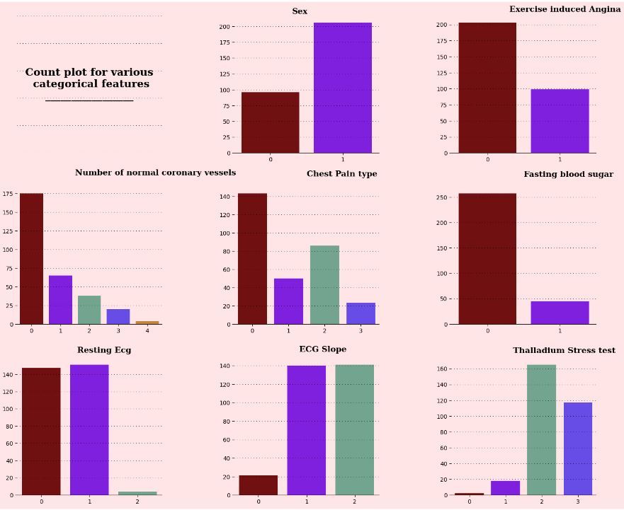
Let’s look at the univariate analysis of categorical variables
fig = plt.figure(figsize=(18,15))
gs = fig.add_gridspec(3,3)
gs.update(wspace=0.5, hspace=0.25)
ax0 = fig.add_subplot(gs[0,0])
ax1 = fig.add_subplot(gs[0,1])
ax2 = fig.add_subplot(gs[0,2])
ax3 = fig.add_subplot(gs[1,0])
ax4 = fig.add_subplot(gs[1,1])
ax5 = fig.add_subplot(gs[1,2])
ax6 = fig.add_subplot(gs[2,0])
ax7 = fig.add_subplot(gs[2,1])
ax8 = fig.add_subplot(gs[2,2])
axes = [ax0,ax1,ax2,ax3,ax4,ax5,ax6,ax7,ax8]
fig.patch.set_facecolor(background_color)
for a in axes:
a.set_facecolor(background_color)
a.grid(color=’#000000′, linestyle=’:’, axis=’y’, zorder=0, dashes=(1,5))
a.set_xlabel(” “)
a.set_ylabel(” “)
for s in [“top”,”right”,’bottom’,”left”]:
ax0.spines[s].set_visible(False)
ax0.tick_params(left=False, bottom=False)
ax0.set_xticklabels([])
ax0.set_yticklabels([])
ax0.text(0.5,0.5,
‘Count plot for various\n categorical features\n_________________’,
horizontalalignment=’center’,
verticalalignment=’center’,
fontsize=18, fontweight=’bold’,
fontfamily=’serif’,
color=”#000000″)
ax1.text(0.3, 220, ‘Sex’, fontsize=14, fontweight=’bold’, fontfamily=’serif’, color=”#000000″)
sns.countplot(ax=ax1,data=df,x=’sex’,palette=color_palette)
ax1.set_xlabel(“”)
ax1.set_ylabel(“”)
ax2.text(0.3, 220, ‘Exercise induced Angina’, fontsize=14, fontweight=’bold’, fontfamily=’serif’, color=”#000000″)
sns.countplot(ax=ax2,data=df,x=’Exercise_induced_Angina’,palette=color_palette)
ax2.set_xlabel(“”)
ax2.set_ylabel(“”)
ax3.text(1.5, 200, ‘Number of normal coronary vessels’, fontsize=14, fontweight=’bold’, fontfamily=’serif’, color=”#000000″)
sns.countplot(ax=ax3,data=df,x=’Coronary_artery_abnormality’,palette=color_palette)
ax3.set_xlabel(“”)
ax3.set_ylabel(“”)
ax4.text(1.5, 162, ‘Chest Pain type’, fontsize=14, fontweight=’bold’, fontfamily=’serif’, color=”#000000″)
sns.countplot(ax=ax4,data=df,x=’Chest_Pain_type’,palette=color_palette)
ax4.set_xlabel(“”)
ax4.set_ylabel(“”)
ax5.text(0.5, 290, ‘Fasting blood sugar’, fontsize=14, fontweight=’bold’, fontfamily=’serif’, color=”#000000″)
sns.countplot(ax=ax5,data=df,x=’Fasting_blood_sugar’,palette=color_palette)
ax5.set_xlabel(“”)
ax5.set_ylabel(“”)
ax6.text(0.75, 165, ‘Resting Ecg’, fontsize=14, fontweight=’bold’, fontfamily=’serif’, color=”#000000″)
sns.countplot(ax=ax6,data=df,x=’Resting_ECG’,palette=color_palette)
ax6.set_xlabel(“”)
ax6.set_ylabel(“”)
ax7.text(0.85, 155, ‘ECG Slope’, fontsize=14, fontweight=’bold’, fontfamily=’serif’, color=”#000000″)
sns.countplot(ax=ax7,data=df,x=’ECG_Slope’,palette=color_palette)
ax7.set_xlabel(“”)
ax7.set_ylabel(“”)
ax8.text(1.2, 180, ‘Thalladium Stress test’, fontsize=14, fontweight=’bold’, fontfamily=’serif’, color=”#000000″)
sns.countplot(ax=ax8,data=df,x=’Thalladium_test’,palette=color_palette)
ax8.set_xlabel(“”)
ax8.set_ylabel(“”)
for s in [“top”,”right”,”left”]:
ax1.spines[s].set_visible(False)
ax2.spines[s].set_visible(False)
ax3.spines[s].set_visible(False)
ax4.spines[s].set_visible(False)
ax5.spines[s].set_visible(False)
ax6.spines[s].set_visible(False)
ax7.spines[s].set_visible(False)
ax8.spines[s].set_visible(False)
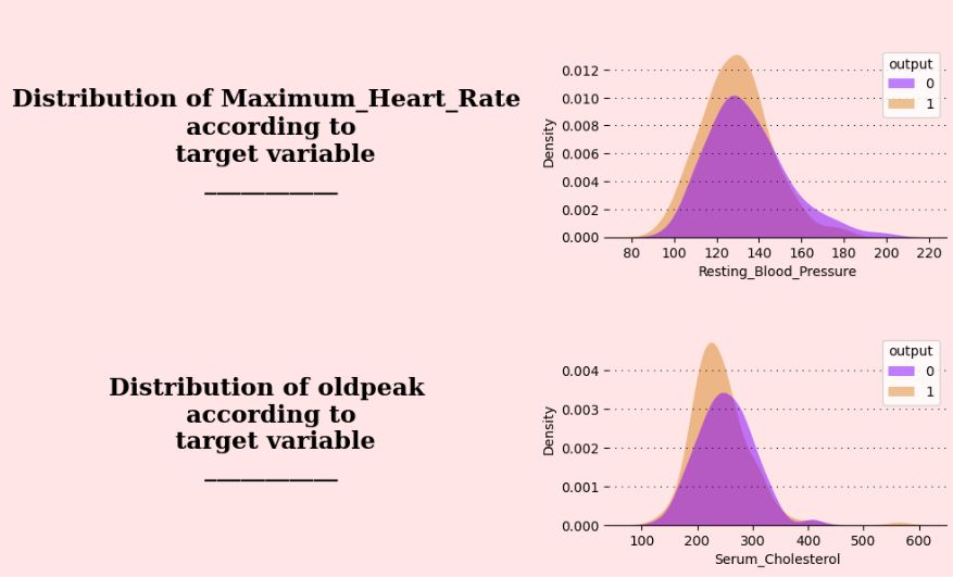
Let’s perform the multivariate analysis of continuous variables
fig = plt.figure(figsize=(18,18))
gs = fig.add_gridspec(5,3)
gs.update(wspace=0.5, hspace=0.5)
ax0 = fig.add_subplot(gs[0,0])
ax1 = fig.add_subplot(gs[0,1])
ax2 = fig.add_subplot(gs[1,0])
ax3 = fig.add_subplot(gs[1,1])
ax4 = fig.add_subplot(gs[2,0])
ax5 = fig.add_subplot(gs[2,1])
ax6 = fig.add_subplot(gs[3,0])
ax7 = fig.add_subplot(gs[3,1])
ax8 = fig.add_subplot(gs[4,0])
ax9 = fig.add_subplot(gs[4,1])
axes = [ax0,ax1,ax2,ax3,ax4,ax5,ax6,ax7,ax8,ax9]
fig.patch.set_facecolor(background_color)
for a in axes:
a.set_facecolor(background_color)
var = [‘Age’,’Resting Blood pressure’,’Serum Cholesterol’,’Maximum_Heart_Rate’,’oldpeak’]
axe = [ax0,ax2,ax4,ax6,ax8]
i = 0
for a in axe:
    a.text(0.5,0.5,"Distribution of " + var[i]+ " \naccording to\n target variable\n___________",
    horizontalalignment = 'center',
    verticalalignment = 'center',
    fontsize = 18,
    fontweight='bold',
    fontfamily='serif',
    color='#000000')
    i = i + 1
    a.spines["bottom"].set_visible(False)
    a.set_xticklabels([])
    a.set_yticklabels([])
    a.tick_params(left=False, bottom=False)
axs = [ax1,ax3,ax5,ax7,ax9]
i = 0
for a in axs:
a.grid(color=’#000000′, linestyle=’:’, axis=’y’, zorder=0, dashes=(1,5))
sns.kdeplot(ax=a, data=df, x =df.columns[i],hue=”output”, fill=True,palette=[“#8000ff”,”#da8829″], alpha=.5, linewidth=0)
i = i + 1
for k in [“top”,”left”,”right”]:
ax0.spines[k].set_visible(False)
ax1.spines[k].set_visible(False)
ax2.spines[k].set_visible(False)
ax3.spines[k].set_visible(False)
ax4.spines[k].set_visible(False)
ax5.spines[k].set_visible(False)
ax6.spines[k].set_visible(False)
ax7.spines[k].set_visible(False)
ax8.spines[k].set_visible(False)
ax9.spines[k].set_visible(False)

Let’s look at the multivariable analysis of categorical features
fig = plt.figure(figsize=(18,20))
gs = fig.add_gridspec(6,3)
gs.update(wspace=0.5, hspace=0.5)
ax0 = fig.add_subplot(gs[0,0])
ax1 = fig.add_subplot(gs[0,1])
ax2 = fig.add_subplot(gs[1,0])
ax3 = fig.add_subplot(gs[1,1])
ax4 = fig.add_subplot(gs[2,0])
ax5 = fig.add_subplot(gs[2,1])
ax6 = fig.add_subplot(gs[3,0])
ax7 = fig.add_subplot(gs[3,1])
ax8 = fig.add_subplot(gs[4,0])
ax9 = fig.add_subplot(gs[4,1])
fig.patch.set_facecolor(background_color)
axes = [ax0,ax1,ax2,ax3,ax4,ax5,ax6,ax7,ax8,ax9]
for a in axes:
a.set_facecolor(background_color)
ax0.text(0.5,0.5,”Chest pain\ndistribution\n__________”,
horizontalalignment = ‘center’,
verticalalignment = ‘center’,
fontsize = 16,
fontweight=’bold’,
fontfamily=’serif’,
)
ax0.spines[“bottom”].set_visible(False)
ax0.set_xticklabels([])
ax0.set_yticklabels([])
ax0.tick_params(left=False, bottom=False)
ax0.text(1,.5,”0 – Typical Angina\n1 – Atypical Angina\n2 – Non-anginal Pain\n3 – Asymptomatic”,
horizontalalignment = ‘center’,
verticalalignment = ‘center’,
fontsize = 14
)
ax1.grid(color=’#000000′, linestyle=’:’, axis=’y’, zorder=0, dashes=(1,5))
sns.kdeplot(ax=ax1, data=df, x=’Chest_Pain_type’,hue=”output”, fill=True,palette=[“#8000ff”,”#da8829″], alpha=.5, linewidth=0)
ax1.set_xlabel(“”)
ax1.set_ylabel(“”)
ax2.text(0.5,0.5,”Number of\nnormal major vessels \n___________”,
horizontalalignment = ‘center’,
verticalalignment = ‘center’,
fontsize = 16,
fontweight=’bold’,
fontfamily=’serif’,
color=’#000000′)
ax2.text(1,.5,”0 vessels\n1 vessel\n2 vessels\n3 vessels\n4 vessels”,
horizontalalignment = ‘center’,
verticalalignment = ‘center’,
fontsize = 14
)
ax2.spines[“bottom”].set_visible(False)
ax2.set_xticklabels([])
ax2.set_yticklabels([])
ax2.tick_params(left=False, bottom=False)
ax3.grid(color=’#000000′, linestyle=’:’, axis=’y’, zorder=0, dashes=(1,5))
sns.kdeplot(ax=ax3, data=df, x=’Coronary_artery_abnormality’,hue=”output”, fill=True,palette=[“#8000ff”,”#da8829″], alpha=.5, linewidth=0)
ax3.set_xlabel(“”)
ax3.set_ylabel(“”)
ax4.text(0.5,0.5,”Coronary artery disease\naccording to\nsex\n______”,
horizontalalignment = ‘center’,
verticalalignment = ‘center’,
fontsize = 16,
fontweight=’bold’,
fontfamily=’serif’,
color=’#000000′)
ax4.text(1,.5,”0 – Female\n1 – Male”,
horizontalalignment = ‘center’,
verticalalignment = ‘center’,
fontsize = 14
)
ax4.spines[“bottom”].set_visible(False)
ax4.set_xticklabels([])
ax4.set_yticklabels([])
ax4.tick_params(left=False, bottom=False)
ax5.grid(color=’#000000′, linestyle=’:’, axis=’y’, zorder=0, dashes=(1,5))
sns.countplot(ax=ax5,data=df,x=’sex’,palette=[“#8000ff”,”#da8829″], hue=’output’)
ax5.set_xlabel(“”)
ax5.set_ylabel(“”)
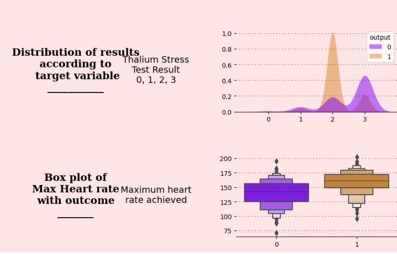
ax6.text(0.5,0.5,”Distribution of results\naccording to\n target variable\n___________”,
horizontalalignment = ‘center’,
verticalalignment = ‘center’,
fontsize = 16,
fontweight=’bold’,
fontfamily=’serif’,
color=’#000000′)
ax6.text(1,.5,”Thalium Stress\nTest Result\n0, 1, 2, 3″,
horizontalalignment = ‘center’,
verticalalignment = ‘center’,
fontsize = 14
)
ax6.spines[“bottom”].set_visible(False)
ax6.set_xticklabels([])
ax6.set_yticklabels([])
ax6.tick_params(left=False, bottom=False)
ax7.grid(color=’#000000′, linestyle=’:’, axis=’y’, zorder=0, dashes=(1,5))
sns.kdeplot(ax=ax7, data=df, x=’Thalladium_test’,hue=”output”, fill=True,palette=[“#8000ff”,”#da8829″], alpha=.5, linewidth=0)
ax7.set_xlabel(“”)
ax7.set_ylabel(“”)
ax8.text(0.5,0.5,”Box plot of\n Max Heart rate \nwith outcome\n_______”,
horizontalalignment = ‘center’,
verticalalignment = ‘center’,
fontsize = 16,
fontweight=’bold’,
fontfamily=’serif’,
color=’#000000′)
ax8.text(1,.5,”Maximum heart\nrate achieved”,
horizontalalignment = ‘center’,
verticalalignment = ‘center’,
fontsize = 14
)
ax8.spines[“bottom”].set_visible(False)
ax8.set_xticklabels([])
ax8.set_yticklabels([])
ax8.tick_params(left=False, bottom=False)
ax9.grid(color=’#000000′, linestyle=’:’, axis=’y’, zorder=0, dashes=(1,5))
sns.boxenplot(ax=ax9, data=df,x=’output’,y=’Maximum_Heart_Rate’,palette=[“#8000ff”,”#da8829″])
ax9.set_xlabel(“”)
ax9.set_ylabel(“”)
for i in [“top”,”left”,”right”]:
ax0.spines[i].set_visible(False)
ax1.spines[i].set_visible(False)
ax2.spines[i].set_visible(False)
ax3.spines[i].set_visible(False)
ax4.spines[i].set_visible(False)
ax5.spines[i].set_visible(False)
ax6.spines[i].set_visible(False)
ax7.spines[i].set_visible(False)
ax8.spines[i].set_visible(False)
ax9.spines[i].set_visible(False)


Let’s look at the multivariable analysis of categorical features
fig = plt.figure(figsize=(18,20))
gs = fig.add_gridspec(6,3)
gs.update(wspace=0.5, hspace=0.5)
ax0 = fig.add_subplot(gs[0,0])
ax1 = fig.add_subplot(gs[0,1])
ax2 = fig.add_subplot(gs[1,0])
ax3 = fig.add_subplot(gs[1,1])
ax4 = fig.add_subplot(gs[2,0])
ax5 = fig.add_subplot(gs[2,1])
ax6 = fig.add_subplot(gs[3,0])
ax7 = fig.add_subplot(gs[3,1])
ax8 = fig.add_subplot(gs[4,0])
ax9 = fig.add_subplot(gs[4,1])
fig.patch.set_facecolor(background_color)
axes = [ax0,ax1,ax2,ax3,ax4,ax5,ax6,ax7,ax8,ax9]
for a in axes:
a.set_facecolor(background_color)
ax0.text(0.5,0.5,”Chest pain\ndistribution\n__________”,
horizontalalignment = ‘center’,
verticalalignment = ‘center’,
fontsize = 16,
fontweight=’bold’,
fontfamily=’serif’,
)
ax0.spines[“bottom”].set_visible(False)
ax0.set_xticklabels([])
ax0.set_yticklabels([])
ax0.tick_params(left=False, bottom=False)
ax0.text(1,.5,”0 – Typical Angina\n1 – Atypical Angina\n2 – Non-anginal Pain\n3 – Asymptomatic”,
horizontalalignment = ‘center’,
verticalalignment = ‘center’,
fontsize = 14
)
ax1.grid(color=’#000000′, linestyle=’:’, axis=’y’, zorder=0, dashes=(1,5))
sns.kdeplot(ax=ax1, data=df, x=’Chest_Pain_type’,hue=”output”, fill=True,palette=[“#8000ff”,”#da8829″], alpha=.5, linewidth=0)
ax1.set_xlabel(“”)
ax1.set_ylabel(“”)
ax2.text(0.5,0.5,”Number of\nnormal major vessels \n___________”,
horizontalalignment = ‘center’,
verticalalignment = ‘center’,
fontsize = 16,
fontweight=’bold’,
fontfamily=’serif’,
color=’#000000′)
ax2.text(1,.5,”0 vessels\n1 vessel\n2 vessels\n3 vessels\n4 vessels”,
horizontalalignment = ‘center’,
verticalalignment = ‘center’,
fontsize = 14
)
ax2.spines[“bottom”].set_visible(False)
ax2.set_xticklabels([])
ax2.set_yticklabels([])
ax2.tick_params(left=False, bottom=False)
ax3.grid(color=’#000000′, linestyle=’:’, axis=’y’, zorder=0, dashes=(1,5))
sns.kdeplot(ax=ax3, data=df, x=’Coronary_artery_abnormality’,hue=”output”, fill=True,palette=[“#8000ff”,”#da8829″], alpha=.5, linewidth=0)
ax3.set_xlabel(“”)
ax3.set_ylabel(“”)
ax4.text(0.5,0.5,”Coronary artery disease\naccording to\nsex\n______”,
horizontalalignment = ‘center’,
verticalalignment = ‘center’,
fontsize = 16,
fontweight=’bold’,
fontfamily=’serif’,
color=’#000000′)
ax4.text(1,.5,”0 – Female\n1 – Male”,
horizontalalignment = ‘center’,
verticalalignment = ‘center’,
fontsize = 14
)
ax4.spines[“bottom”].set_visible(False)
ax4.set_xticklabels([])
ax4.set_yticklabels([])
ax4.tick_params(left=False, bottom=False)
ax5.grid(color=’#000000′, linestyle=’:’, axis=’y’, zorder=0, dashes=(1,5))
sns.countplot(ax=ax5,data=df,x=’sex’,palette=[“#8000ff”,”#da8829″], hue=’output’)
ax5.set_xlabel(“”)
ax5.set_ylabel(“”)
ax6.text(0.5,0.5,”Distribution of results\naccording to\n target variable\n___________”,
horizontalalignment = ‘center’,
verticalalignment = ‘center’,
fontsize = 16,
fontweight=’bold’,
fontfamily=’serif’,
color=’#000000′)
ax6.text(1,.5,”Thalium Stress\nTest Result\n0, 1, 2, 3″,
horizontalalignment = ‘center’,
verticalalignment = ‘center’,
fontsize = 14
)
ax6.spines[“bottom”].set_visible(False)
ax6.set_xticklabels([])
ax6.set_yticklabels([])
ax6.tick_params(left=False, bottom=False)
ax7.grid(color=’#000000′, linestyle=’:’, axis=’y’, zorder=0, dashes=(1,5))
sns.kdeplot(ax=ax7, data=df, x=’Thalladium_test’,hue=”output”, fill=True,palette=[“#8000ff”,”#da8829″], alpha=.5, linewidth=0)
ax7.set_xlabel(“”)
ax7.set_ylabel(“”)
ax8.text(0.5,0.5,”Box plot of\n Max Heart rate \nwith outcome\n_______”,
horizontalalignment = ‘center’,
verticalalignment = ‘center’,
fontsize = 16,
fontweight=’bold’,
fontfamily=’serif’,
color=’#000000′)
ax8.text(1,.5,”Maximum heart\nrate achieved”,
horizontalalignment = ‘center’,
verticalalignment = ‘center’,
fontsize = 14
)
ax8.spines[“bottom”].set_visible(False)
ax8.set_xticklabels([])
ax8.set_yticklabels([])
ax8.tick_params(left=False, bottom=False)
ax9.grid(color=’#000000′, linestyle=’:’, axis=’y’, zorder=0, dashes=(1,5))
sns.boxenplot(ax=ax9, data=df,x=’output’,y=’Maximum_Heart_Rate’,palette=[“#8000ff”,”#da8829″])
ax9.set_xlabel(“”)
ax9.set_ylabel(“”)
for i in [“top”,”left”,”right”]:
ax0.spines[i].set_visible(False)
ax1.spines[i].set_visible(False)
ax2.spines[i].set_visible(False)
ax3.spines[i].set_visible(False)
ax4.spines[i].set_visible(False)
ax5.spines[i].set_visible(False)
ax6.spines[i].set_visible(False)
ax7.spines[i].set_visible(False)
ax8.spines[i].set_visible(False)
ax9.spines[i].set_visible(False)

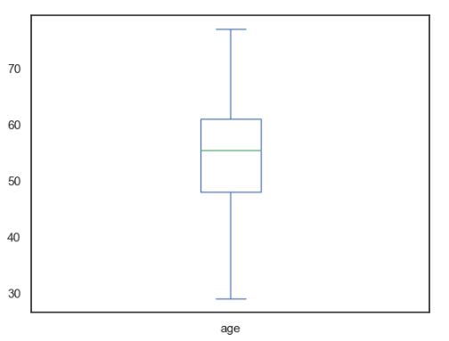
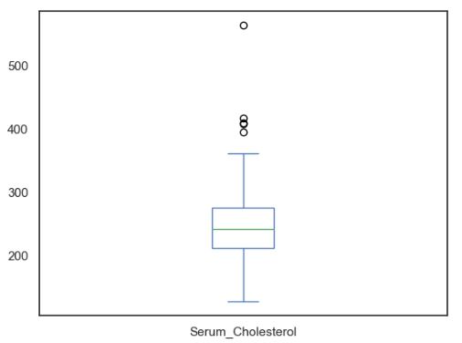
Let’s look at boxplots of individual features
dataset = df
dataset[‘age’].plot(kind=’box’, subplots=True, sharex=False, sharey=False)
plt.figure()
dataset[‘Resting_Blood_Pressure’].plot(kind=’box’, subplots=True, sharex=False, sharey=False)
plt.figure()

dataset[‘Serum_Cholesterol’].plot(kind=’box’, subplots=True, sharex=False, sharey=False)
plt.figure()
dataset[‘Maximum_Heart_Rate’].plot(kind=’box’, subplots=True, sharex=False, sharey=False)
plt.figure()

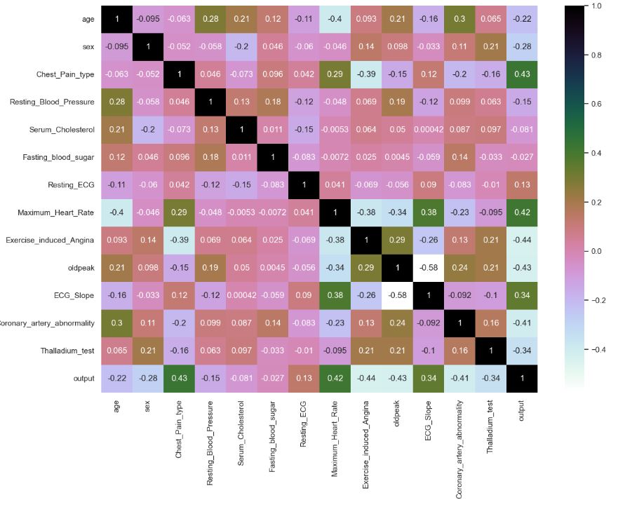
Feature Correlations
Let’s plot the feature correlation matrix heatmap
plt.figure(figsize=(14,10))
sns.heatmap(dataset.corr(),annot=True,cmap=’cubehelix_r’)
plt.show()
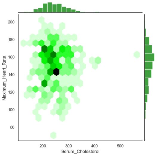
Let’s compare the seaborn hexagonal bin plots
sns.jointplot(x=”age”, y=”Maximum_Heart_Rate”, data=dataset, ratio=10, kind=’hex’,color=’green’)
plt.show()

sns.jointplot(x=”Serum_Cholesterol”, y=”Maximum_Heart_Rate”, data=dataset, ratio=10, kind=’hex’,color=’green’)
plt.show()
sns.jointplot(x=”Resting_Blood_Pressure”, y=”Maximum_Heart_Rate”, data=dataset, ratio=10, kind=’hex’,color=’green’)
plt.show()

sns.jointplot(x=”Resting_Blood_Pressure”, y=”Serum_Cholesterol”, data=dataset, ratio=10, kind=’hex’,color=’green’)
plt.show()

sns.jointplot(x=”Resting_Blood_Pressure”, y=”age”, data=dataset, ratio=10, kind=’hex’,color=’green’)
plt.show()

Multiple ML/AI Models
Let’s import the libraries
from sklearn.ensemble import RandomForestClassifier
from sklearn.neighbors import KNeighborsClassifier
from sklearn.linear_model import LogisticRegression
from sklearn.preprocessing import StandardScaler
from sklearn.svm import SVC
from sklearn.metrics import accuracy_score
from sklearn.model_selection import train_test_split
from sklearn.metrics import precision_score,recall_score
from sklearn.metrics import f1_score
from sklearn.metrics import confusion_matrix,accuracy_score, classification_report
from sklearn.metrics import ConfusionMatrixDisplay
and prepare the input data
df1 = df
let’s define the columns to be encoded and scaled
cat_cols = [‘Coronary_artery_abnormality’,’Chest_Pain_type’,’Resting_ECG’,’ECG_Slope’,’Thalladium_test’]
con_cols = [“age”,”Resting_Blood_Pressure”,”Serum_Cholesterol”,”Maximum_Heart_Rate”,”oldpeak”]
encoding the categorical columns
df1 = pd.get_dummies(df1, columns = cat_cols, drop_first = True)
and defining the features and target
X = df1.drop([‘output’],axis=1)
y = df1[[‘output’]]
Let’s perform train_test_split with test_size = 0.2
X_train, X_test, y_train, y_test = train_test_split(X,y, test_size = 0.2, random_state = 42)
instantiating the scaler
scaler =StandardScaler()
and scaling the continuous features
d = scaler.fit_transform(X_train)
X_test = scaler.transform(X_test)
names = X.columns
scaled = pd.DataFrame(d, columns=names)
#scaled.head()
Let’s begin training the most popular models
models = [RandomForestClassifier(), KNeighborsClassifier(), SVC(), LogisticRegression()]
for a in models:
a.fit(X_train, y_train)
y_pred = a.predict(X_test)
a = print(f'model: {str(a)}')
b= print(classification_report(y_test,y_pred, zero_division=1))
c = print('-'*30, '\n')
model: RandomForestClassifier()
              precision    recall  f1-score   support

           0       0.78      0.86      0.82        29
           1       0.86      0.78      0.82        32

    accuracy                           0.82        61
   macro avg       0.82      0.82      0.82        61
weighted avg       0.82      0.82      0.82        61

------------------------------

model: KNeighborsClassifier()
              precision    recall  f1-score   support

           0       0.48      1.00      0.64        29
           1       1.00      0.00      0.00        32

    accuracy                           0.48        61
   macro avg       0.74      0.50      0.32        61
weighted avg       0.75      0.48      0.31        61

------------------------------

model: SVC()
              precision    recall  f1-score   support

           0       0.48      1.00      0.64        29
           1       1.00      0.00      0.00        32

    accuracy                           0.48        61
   macro avg       0.74      0.50      0.32        61
weighted avg       0.75      0.48      0.31        61

------------------------------

model: LogisticRegression()
              precision    recall  f1-score   support

           0       0.79      0.90      0.84        29
           1       0.89      0.78      0.83        32

    accuracy                           0.84        61
   macro avg       0.84      0.84      0.84        61
weighted avg       0.84      0.84      0.84        61

------------------------------
Feature Importance
Let’s select RandomForestClassifier
FinalM= RandomForestClassifier()
FinalM.fit(X_train, y_train)
y_pred = FinalM.predict(X_test)
print(classification_report(y_test,y_pred, zero_division=1))
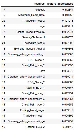
feature_importances=FinalM.feature_importances_
feature_importances_df=pd.DataFrame({‘features’:list(X_train), ‘feature_importances’:feature_importances})
feature_importances_df=pd.DataFrame({‘features’:list(X_train), ‘feature_importances’:feature_importances})
feature_importances_df.sort_values(‘feature_importances’,ascending=False)
   precision    recall  f1-score   support

           0       0.86      0.83      0.84        29
           1       0.85      0.88      0.86        32

    accuracy                           0.85        61
   macro avg       0.85      0.85      0.85        61
weighted avg       0.85      0.85      0.85        61
Let’s visualize this table as a vertical bar plot
plt.figure(figsize=(20,15))
importance = FinalM.feature_importances_
idxs = np.argsort(importance, axis=0, order=None)
sort = np.sort(idxs)
new = sort[:15]
ax = plt.axes()
ax.set_facecolor(background_color)
plt.title(“Feature Importance”,fontsize=30)
plt.barh(range(len(new)),importance[new],align=”center”,color = color_palette)
plt.yticks(range(len(new)),(feature_importances_df[‘features’][i] for i in new),fontsize=20)
plt.xlabel(“Random Forest Feature Importance”,fontsize=18)
plt.tight_layout()
plt.show()

Model Performance
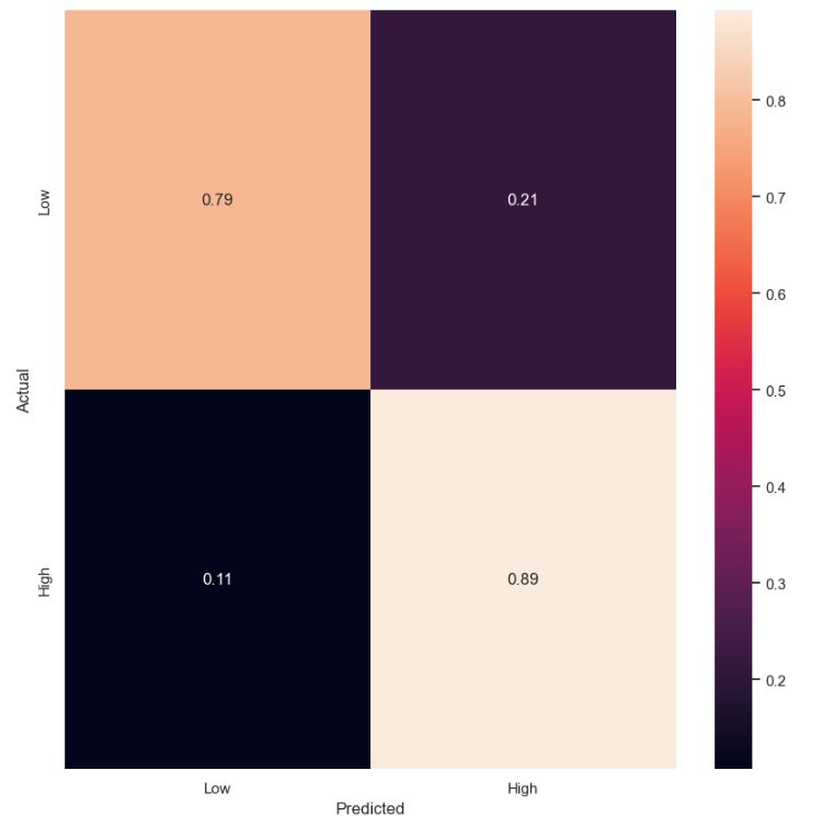
Let’s select LogisticRegression and plot both classification report and the normalized confusion matrix
FinalM= LogisticRegression()
FinalM.fit(X_train, y_train)
y_pred = FinalM.predict(X_test)
print(classification_report(y_test,y_pred, zero_division=1))
   precision    recall  f1-score   support

           0       0.79      0.90      0.84        29
           1       0.89      0.78      0.83        32

    accuracy                           0.84        61
   macro avg       0.84      0.84      0.84        61
weighted avg       0.84      0.84      0.84        61
cm = confusion_matrix(FinalM.predict(X_test),y_test)
target_names=[‘Low’,’High’]
cmn = cm.astype(‘float’) / cm.sum(axis=1)[:, np.newaxis]
fig, ax = plt.subplots(figsize=(10,10))
sns.heatmap(cmn, annot=True, fmt=’.2f’, xticklabels=target_names, yticklabels=target_names)
plt.ylabel(‘Actual’)
plt.xlabel(‘Predicted’)
plt.show(block=False)

Let’s select RandomForestClassifier
FinalM= RandomForestClassifier()
FinalM.fit(X_train, y_train)
y_pred = FinalM.predict(X_test)
print(classification_report(y_test,y_pred, zero_division=1))
precision    recall  f1-score   support

           0       0.86      0.83      0.84        29
           1       0.85      0.88      0.86        32

    accuracy                           0.85        61
   macro avg       0.85      0.85      0.85        61
weighted avg       0.85      0.85      0.85        61
and plot the normalized confusion matrix
cm = confusion_matrix(FinalM.predict(X_test),y_test)
target_names=[‘Low’,’High’]
cmn = cm.astype(‘float’) / cm.sum(axis=1)[:, np.newaxis]
fig, ax = plt.subplots(figsize=(10,10))
sns.heatmap(cmn, annot=True, fmt=’.2f’, xticklabels=target_names, yticklabels=target_names)
plt.ylabel(‘Actual’)
plt.xlabel(‘Predicted’)
plt.show(block=False)

Let’s look at all estimators
from sklearn.utils import all_estimators
estimators = all_estimators(type_filter=’classifier’)
all_clfs = []
for name, ClassifierClass in estimators:
print(‘Appending’, name)
try:
clf = ClassifierClass()
all_clfs.append(clf)
except Exception as e:
print(‘Unable to import’, name)
print(e)
Appending AdaBoostClassifier
Appending BaggingClassifier
Appending BernoulliNB
Appending CalibratedClassifierCV
Appending CategoricalNB
Appending ClassifierChain
Unable to import ClassifierChain
__init__() missing 1 required positional argument: 'base_estimator'
Appending ComplementNB
Appending DecisionTreeClassifier
Appending DummyClassifier
Appending ExtraTreeClassifier
Appending ExtraTreesClassifier
Appending GaussianNB
Appending GaussianProcessClassifier
Appending GradientBoostingClassifier
Appending HistGradientBoostingClassifier
Appending KNeighborsClassifier
Appending LabelPropagation
Appending LabelSpreading
Appending LinearDiscriminantAnalysis
Appending LinearSVC
Appending LogisticRegression
Appending LogisticRegressionCV
Appending MLPClassifier
Appending MultiOutputClassifier
Unable to import MultiOutputClassifier
__init__() missing 1 required positional argument: 'estimator'
Appending MultinomialNB
Appending NearestCentroid
Appending NuSVC
Appending OneVsOneClassifier
Unable to import OneVsOneClassifier
__init__() missing 1 required positional argument: 'estimator'
Appending OneVsRestClassifier
Unable to import OneVsRestClassifier
__init__() missing 1 required positional argument: 'estimator'
Appending OutputCodeClassifier
Unable to import OutputCodeClassifier
__init__() missing 1 required positional argument: 'estimator'
Appending PassiveAggressiveClassifier
Appending Perceptron
Appending QuadraticDiscriminantAnalysis
Appending RadiusNeighborsClassifier
Appending RandomForestClassifier
Appending RidgeClassifier
Appending RidgeClassifierCV
Appending SGDClassifier
Appending SVC
Appending StackingClassifier
Unable to import StackingClassifier
__init__() missing 1 required positional argument: 'estimators'
Appending VotingClassifier
Unable to import VotingClassifier
__init__() missing 1 required positional argument: 'estimators'
print (all_clfs)
[AdaBoostClassifier(), BaggingClassifier(), BernoulliNB(), CalibratedClassifierCV(), CategoricalNB(), ComplementNB(), DecisionTreeClassifier(), DummyClassifier(), ExtraTreeClassifier(), ExtraTreesClassifier(), GaussianNB(), GaussianProcessClassifier(), GradientBoostingClassifier(), HistGradientBoostingClassifier(), KNeighborsClassifier(), LabelPropagation(), LabelSpreading(), LinearDiscriminantAnalysis(), LinearSVC(), LogisticRegression(), LogisticRegressionCV(), MLPClassifier(), MultinomialNB(), NearestCentroid(), NuSVC(), PassiveAggressiveClassifier(), Perceptron(), QuadraticDiscriminantAnalysis(), RadiusNeighborsClassifier(), RandomForestClassifier(), RidgeClassifier(), RidgeClassifierCV(), SGDClassifier(), SVC()]
Let’s import libraries and create multiple model pipelines
import xgboost as xgb
import lightgbm as lgb
from sklearn.ensemble import AdaBoostClassifier,BaggingClassifier,ExtraTreesClassifier,GradientBoostingClassifier,HistGradientBoostingClassifier
from sklearn.ensemble import StackingClassifier
from sklearn.naive_bayes import BernoulliNB,ComplementNB,GaussianNB,MultinomialNB
from sklearn.calibration import CalibratedClassifierCV
from sklearn.tree import DecisionTreeClassifier,ExtraTreeClassifier
from sklearn.dummy import DummyClassifier
from sklearn.gaussian_process import GaussianProcessClassifier
from sklearn.semi_supervised import LabelPropagation,LabelSpreading
from sklearn.discriminant_analysis import LinearDiscriminantAnalysis
from sklearn.svm import LinearSVC,NuSVC
from sklearn.linear_model import LogisticRegressionCV,PassiveAggressiveClassifier,Perceptron,RidgeClassifier,RidgeClassifierCV
from sklearn.linear_model import SGDClassifier
from sklearn.neural_network import MLPClassifier
from sklearn.neighbors import NearestCentroid
from sklearn.discriminant_analysis import QuadraticDiscriminantAnalysis
from sklearn.multiclass import OutputCodeClassifier,OneVsRestClassifier
from sklearn.multioutput import ClassifierChain
from sklearn.kernel_approximation import RBFSampler
allclfs = []
clf = AdaBoostClassifier()
allclfs.append(clf)
clf = BaggingClassifier()
allclfs.append(clf)
clf = CalibratedClassifierCV()
allclfs.append(clf)
import numpy as np
from sklearn.pipeline import Pipeline
from sklearn.feature_extraction.text import CountVectorizer
from sklearn.svm import LinearSVC
from sklearn.feature_extraction.text import TfidfTransformer
from sklearn.multiclass import OneVsRestClassifier
classifier = Pipeline([
(‘tfidf’, TfidfTransformer()),
(‘clf’, OneVsRestClassifier(LinearSVC()))])
base_lr = LogisticRegression()
chains = [ClassifierChain(base_lr, order=”random”, random_state=i) for i in range(10)]
forest = RandomForestClassifier(n_estimators=100,
random_state=123)
boost = xgb.XGBClassifier(random_state=123, verbosity=0, use_label_encoder=False)
lgclassifier = LogisticRegression(random_state=123)
estimators = [
(‘rf’, forest),
(‘xgb’, boost)
]
stackclf = StackingClassifier(estimators=estimators,
final_estimator=lgclassifier,
cv=10)
svm = LinearSVC(random_state=42)
ecoc_classifier = OutputCodeClassifier(svm, code_size=6)
from sklearn.ensemble import VotingClassifier
from sklearn.linear_model import LogisticRegression
from sklearn.svm import SVC
from sklearn.tree import DecisionTreeClassifier
estimator = []
estimator.append((‘LR’,
LogisticRegression(solver =’lbfgs’,
multi_class =’multinomial’,
max_iter = 200)))
estimator.append((‘SVC’, SVC(gamma =’auto’, probability = True)))
estimator.append((‘DTC’, DecisionTreeClassifier()))
vot_hard = VotingClassifier(estimators = estimator, voting =’hard’)
vot_soft = VotingClassifier(estimators = estimator, voting =’soft’)
Expanded list of models:
models = [AdaBoostClassifier(), BaggingClassifier(), CalibratedClassifierCV(),ComplementNB(),DecisionTreeClassifier(),DummyClassifier(),
ExtraTreeClassifier(),ExtraTreesClassifier(),GaussianNB(),GaussianProcessClassifier(),GradientBoostingClassifier(),
HistGradientBoostingClassifier(),LabelPropagation(),LabelSpreading(),LinearDiscriminantAnalysis(),LinearSVC(),
LogisticRegressionCV(),MLPClassifier(),MultinomialNB(),NearestCentroid(),NuSVC(),PassiveAggressiveClassifier(),
Perceptron(),QuadraticDiscriminantAnalysis(),xgb.XGBClassifier(),lgb.LGBMClassifier(),RidgeClassifier(),
RidgeClassifierCV(),SGDClassifier(),stackclf,vot_hard,vot_soft,ecoc_classifier,classifier]
for a in models:
a.fit(X_train, y_train)
y_pred = a.predict(X_test)
a = print(f'model: {str(a)}')
b= print(classification_report(y_test,y_pred, zero_division=1))
c = print('-'*30, '\n')
model: AdaBoostClassifier()
              precision    recall  f1-score   support

           0       0.62      0.97      0.76        29
           1       0.94      0.47      0.62        32

    accuracy                           0.70        61
   macro avg       0.78      0.72      0.69        61
weighted avg       0.79      0.70      0.69        61

------------------------------
model: BaggingClassifier()
              precision    recall  f1-score   support

           0       0.60      0.62      0.61        29
           1       0.65      0.62      0.63        32

    accuracy                           0.62        61
   macro avg       0.62      0.62      0.62        61
weighted avg       0.62      0.62      0.62        61

------------------------------

model: CalibratedClassifierCV()
              precision    recall  f1-score   support

           0       0.91      0.69      0.78        29
           1       0.77      0.94      0.85        32

    accuracy                           0.82        61
   macro avg       0.84      0.81      0.81        61
weighted avg       0.84      0.82      0.82        61

------------------------------

model: ComplementNB()
              precision    recall  f1-score   support

           0       0.78      0.86      0.82        29
           1       0.86      0.78      0.82        32

    accuracy                           0.82        61
   macro avg       0.82      0.82      0.82        61
weighted avg       0.82      0.82      0.82        61

------------------------------

model: DecisionTreeClassifier()
              precision    recall  f1-score   support

           0       0.56      0.76      0.65        29
           1       0.68      0.47      0.56        32

    accuracy                           0.61        61
   macro avg       0.62      0.61      0.60        61
weighted avg       0.63      0.61      0.60        61

------------------------------

model: DummyClassifier()
              precision    recall  f1-score   support

           0       1.00      0.00      0.00        29
           1       0.52      1.00      0.69        32

    accuracy                           0.52        61
   macro avg       0.76      0.50      0.34        61
weighted avg       0.75      0.52      0.36        61

------------------------------

model: ExtraTreeClassifier()
              precision    recall  f1-score   support

           0       0.64      0.24      0.35        29
           1       0.56      0.88      0.68        32

    accuracy                           0.57        61
   macro avg       0.60      0.56      0.52        61
weighted avg       0.60      0.57      0.52        61

------------------------------

model: ExtraTreesClassifier()
              precision    recall  f1-score   support

           0       0.81      0.86      0.83        29
           1       0.87      0.81      0.84        32

    accuracy                           0.84        61
   macro avg       0.84      0.84      0.84        61
weighted avg       0.84      0.84      0.84        61

------------------------------

model: GaussianNB()
              precision    recall  f1-score   support

           0       0.58      1.00      0.73        29
           1       1.00      0.34      0.51        32

    accuracy                           0.66        61
   macro avg       0.79      0.67      0.62        61
weighted avg       0.80      0.66      0.62        61

------------------------------

model: GaussianProcessClassifier()
              precision    recall  f1-score   support

           0       0.48      1.00      0.64        29
           1       1.00      0.00      0.00        32

    accuracy                           0.48        61
   macro avg       0.74      0.50      0.32        61
weighted avg       0.75      0.48      0.31        61

------------------------------

model: GradientBoostingClassifier()
              precision    recall  f1-score   support

           0       0.63      0.83      0.72        29
           1       0.78      0.56      0.65        32

    accuracy                           0.69        61
   macro avg       0.71      0.70      0.69        61
weighted avg       0.71      0.69      0.68        61

------------------------------

model: HistGradientBoostingClassifier()
              precision    recall  f1-score   support

           0       0.68      0.86      0.76        29
           1       0.83      0.62      0.71        32

    accuracy                           0.74        61
   macro avg       0.75      0.74      0.74        61
weighted avg       0.76      0.74      0.73        61

------------------------------

model: LabelPropagation()
              precision    recall  f1-score   support

           0       0.48      1.00      0.64        29
           1       1.00      0.00      0.00        32

    accuracy                           0.48        61
   macro avg       0.74      0.50      0.32        61
weighted avg       0.75      0.48      0.31        61

------------------------------

model: LabelSpreading()
              precision    recall  f1-score   support

           0       0.48      1.00      0.64        29
           1       1.00      0.00      0.00        32

    accuracy                           0.48        61
   macro avg       0.74      0.50      0.32        61
weighted avg       0.75      0.48      0.31        61

------------------------------

model: LinearDiscriminantAnalysis()
              precision    recall  f1-score   support

           0       0.92      0.83      0.87        29
           1       0.86      0.94      0.90        32

    accuracy                           0.89        61
   macro avg       0.89      0.88      0.88        61
weighted avg       0.89      0.89      0.88        61

------------------------------

model: LinearSVC()
              precision    recall  f1-score   support

           0       0.78      0.86      0.82        29
           1       0.86      0.78      0.82        32

    accuracy                           0.82        61
   macro avg       0.82      0.82      0.82        61
weighted avg       0.82      0.82      0.82        61

------------------------------

model: LogisticRegressionCV()
              precision    recall  f1-score   support

           0       0.82      0.97      0.89        29
           1       0.96      0.81      0.88        32

    accuracy                           0.89        61
   macro avg       0.89      0.89      0.89        61
weighted avg       0.90      0.89      0.88        61

------------------------------

model: MLPClassifier()
              precision    recall  f1-score   support

           0       0.81      0.86      0.83        29
           1       0.87      0.81      0.84        32

    accuracy                           0.84        61
   macro avg       0.84      0.84      0.84        61
weighted avg       0.84      0.84      0.84        61

------------------------------

model: MultinomialNB()
              precision    recall  f1-score   support

           0       0.78      0.86      0.82        29
           1       0.86      0.78      0.82        32

    accuracy                           0.82        61
   macro avg       0.82      0.82      0.82        61
weighted avg       0.82      0.82      0.82        61

------------------------------

model: NearestCentroid()
              precision    recall  f1-score   support

           0       0.48      1.00      0.64        29
           1       1.00      0.00      0.00        32

    accuracy                           0.48        61
   macro avg       0.74      0.50      0.32        61
weighted avg       0.75      0.48      0.31        61

------------------------------

model: NuSVC()
              precision    recall  f1-score   support

           0       0.48      1.00      0.64        29
           1       1.00      0.00      0.00        32

    accuracy                           0.48        61
   macro avg       0.74      0.50      0.32        61
weighted avg       0.75      0.48      0.31        61

------------------------------

model: PassiveAggressiveClassifier()
              precision    recall  f1-score   support

           0       0.78      0.86      0.82        29
           1       0.86      0.78      0.82        32

    accuracy                           0.82        61
   macro avg       0.82      0.82      0.82        61
weighted avg       0.82      0.82      0.82        61

------------------------------

model: Perceptron()
              precision    recall  f1-score   support

           0       0.74      0.79      0.77        29
           1       0.80      0.75      0.77        32

    accuracy                           0.77        61
   macro avg       0.77      0.77      0.77        61
weighted avg       0.77      0.77      0.77        61

------------------------------

model: QuadraticDiscriminantAnalysis()
              precision    recall  f1-score   support

           0       1.00      0.00      0.00        29
           1       0.52      1.00      0.69        32

    accuracy                           0.52        61
   macro avg       0.76      0.50      0.34        61
weighted avg       0.75      0.52      0.36        61

------------------------------
model: XGBClassifier(base_score=0.5, booster='gbtree', callbacks=None,
              colsample_bylevel=1, colsample_bynode=1, colsample_bytree=1,
              early_stopping_rounds=None, enable_categorical=False,
              eval_metric=None, feature_types=None, gamma=0, gpu_id=-1,
              grow_policy='depthwise', importance_type=None,
              interaction_constraints='', learning_rate=0.300000012,
              max_bin=256, max_cat_threshold=64, max_cat_to_onehot=4,
              max_delta_step=0, max_depth=6, max_leaves=0, min_child_weight=1,
              missing=nan, monotone_constraints='()', n_estimators=100,
              n_jobs=0, num_parallel_tree=1, predictor='auto', random_state=0, ...)
              precision    recall  f1-score   support

           0       0.68      0.79      0.73        29
           1       0.78      0.66      0.71        32

    accuracy                           0.72        61
   macro avg       0.73      0.72      0.72        61
weighted avg       0.73      0.72      0.72        61

------------------------------

model: LGBMClassifier()
              precision    recall  f1-score   support

           0       0.67      0.90      0.76        29
           1       0.86      0.59      0.70        32

    accuracy                           0.74        61
   macro avg       0.77      0.75      0.73        61
weighted avg       0.77      0.74      0.73        61

------------------------------

model: RidgeClassifier()
              precision    recall  f1-score   support

           0       0.93      0.86      0.89        29
           1       0.88      0.94      0.91        32

    accuracy                           0.90        61
   macro avg       0.90      0.90      0.90        61
weighted avg       0.90      0.90      0.90        61

------------------------------

model: RidgeClassifierCV()
              precision    recall  f1-score   support

           0       0.93      0.86      0.89        29
           1       0.88      0.94      0.91        32

    accuracy                           0.90        61
   macro avg       0.90      0.90      0.90        61
weighted avg       0.90      0.90      0.90        61

------------------------------

model: SGDClassifier()
              precision    recall  f1-score   support

           0       0.74      0.90      0.81        29
           1       0.88      0.72      0.79        32

    accuracy                           0.80        61
   macro avg       0.81      0.81      0.80        61
weighted avg       0.82      0.80      0.80        61

------------------------------

model: StackingClassifier(cv=10,
                   estimators=[('rf', RandomForestClassifier(random_state=123)),
                               ('xgb',
                                XGBClassifier(base_score=None, booster=None,
                                              callbacks=None,
                                              colsample_bylevel=None,
                                              colsample_bynode=None,
                                              colsample_bytree=None,
                                              early_stopping_rounds=None,
                                              enable_categorical=False,
                                              eval_metric=None,
                                              feature_types=None, gamma=None,
                                              gpu_id=None, grow_policy=None,
                                              impor...
                                              interaction_constraints=None,
                                              learning_rate=None, max_bin=None,
                                              max_cat_threshold=None,
                                              max_cat_to_onehot=None,
                                              max_delta_step=None,
                                              max_depth=None, max_leaves=None,
                                              min_child_weight=None,
                                              missing=nan,
                                              monotone_constraints=None,
                                              n_estimators=100, n_jobs=None,
                                              num_parallel_tree=None,
                                              predictor=None, random_state=123, ...))],
                   final_estimator=LogisticRegression(random_state=123))
              precision    recall  f1-score   support

           0       0.76      0.86      0.81        29
           1       0.86      0.75      0.80        32

    accuracy                           0.80        61
   macro avg       0.81      0.81      0.80        61
weighted avg       0.81      0.80      0.80        61

------------------------------

model: VotingClassifier(estimators=[('LR',
                              LogisticRegression(max_iter=200,
                                                 multi_class='multinomial')),
                             ('SVC', SVC(gamma='auto', probability=True)),
                             ('DTC', DecisionTreeClassifier())])
              precision    recall  f1-score   support

           0       0.96      0.76      0.85        29
           1       0.82      0.97      0.89        32

    accuracy                           0.87        61
   macro avg       0.89      0.86      0.87        61
weighted avg       0.88      0.87      0.87        61

------------------------------

model: VotingClassifier(estimators=[('LR',
                              LogisticRegression(max_iter=200,
                                                 multi_class='multinomial')),
                             ('SVC', SVC(gamma='auto', probability=True)),
                             ('DTC', DecisionTreeClassifier())],
                 voting='soft')
              precision    recall  f1-score   support

           0       0.87      0.45      0.59        29
           1       0.65      0.94      0.77        32

    accuracy                           0.70        61
   macro avg       0.76      0.69      0.68        61
weighted avg       0.75      0.70      0.68        61

------------------------------

model: OutputCodeClassifier(code_size=6, estimator=LinearSVC(random_state=42))
              precision    recall  f1-score   support

           0       0.78      0.86      0.82        29
           1       0.86      0.78      0.82        32

    accuracy                           0.82        61
   macro avg       0.82      0.82      0.82        61
weighted avg       0.82      0.82      0.82        61

------------------------------

model: Pipeline(steps=[('tfidf', TfidfTransformer()),
                ('clf', OneVsRestClassifier(estimator=LinearSVC()))])
              precision    recall  f1-score   support

           0       0.81      0.90      0.85        29
           1       0.90      0.81      0.85        32

    accuracy                           0.85        61
   macro avg       0.85      0.85      0.85        61
weighted avg       0.86      0.85      0.85        61

------------------------------
Application of all Machine Learning methods:
import sklearn
MLA = [
#GLM
sklearn.linear_model.LogisticRegressionCV(),
sklearn.linear_model.PassiveAggressiveClassifier(),
sklearn.linear_model. RidgeClassifierCV(),
sklearn.linear_model.SGDClassifier(),
sklearn.linear_model.Perceptron(),
#Ensemble Methods
sklearn.ensemble.AdaBoostClassifier(),
sklearn.ensemble.BaggingClassifier(),
sklearn.ensemble.ExtraTreesClassifier(),
sklearn.ensemble.GradientBoostingClassifier(),
sklearn.ensemble.RandomForestClassifier(),

#Gaussian Processes
sklearn.gaussian_process.GaussianProcessClassifier(),

#SVM
sklearn.svm.SVC(probability=True),
sklearn.svm.NuSVC(probability=True),
sklearn.svm.LinearSVC(),

#Trees
sklearn.tree.DecisionTreeClassifier(),

#Navies Bayes
sklearn.naive_bayes.BernoulliNB(),
sklearn.naive_bayes.GaussianNB(),

#Nearest Neighbor
sklearn.neighbors.KNeighborsClassifier(),
]
MLA_columns = []
MLA_compare = pd.DataFrame(columns = MLA_columns)
row_index = 0
for alg in MLA:
predicted = alg.fit(X_train, y_train).predict(X_test)
fp, tp, th = sklearn.metrics.roc_curve(y_test, predicted)
MLA_name = alg.__class__.__name__
MLA_compare.loc[row_index,'MLA used'] = MLA_name
MLA_compare.loc[row_index, 'Train Accuracy'] = round(alg.score(X_train, y_train), 4)
MLA_compare.loc[row_index, 'Test Accuracy'] = round(alg.score(X_test, y_test), 4)
MLA_compare.loc[row_index, 'Precission'] = sklearn.metrics.precision_score(y_test, predicted)
MLA_compare.loc[row_index, 'Recall'] = sklearn.metrics.recall_score(y_test, predicted)
MLA_compare.loc[row_index, 'AUC'] = sklearn.metrics.auc(fp, tp)

row_index+=1
MLA_compare.sort_values(by = [‘Test Accuracy’], ascending = False, inplace = True)
MLA_compare

Let’s perform MLA Train Accuracy Comparison
plt.subplots(figsize=(13,5))
sns.barplot(x=”MLA used”, y=”Train Accuracy”,data=MLA_compare,palette=’hot’,edgecolor=sns.color_palette(‘dark’,7))
plt.xticks(rotation=90)
plt.title(‘MLA Train Accuracy Comparison’)
plt.show()

Let’s check the test data accuracy
plt.subplots(figsize=(13,5))
sns.barplot(x=”MLA used”, y=”Test Accuracy”,data=MLA_compare,palette=’hot’,edgecolor=sns.color_palette(‘dark’,7))
plt.xticks(rotation=90)
plt.title(‘Accuracy of different machine learning models’)
plt.show()

Creating plots to compare precision of the MLAs
plt.subplots(figsize=(13,5))
sns.barplot(x=”MLA used”, y=”Precision”,data=MLA_compare,palette=’hot’,edgecolor=sns.color_palette(‘dark’,7))
plt.xticks(rotation=90)
plt.title(‘Comparing different Machine Learning Models’)
plt.show()

Creating plots for MLA recall comparison
plt.subplots(figsize=(13,5))
sns.barplot(x=”MLA used”, y=”Recall”,data=MLA_compare,palette=’hot’,edgecolor=sns.color_palette(‘dark’,7))
plt.xticks(rotation=90)
plt.title(‘MLA Recall Comparison’)
plt.show()

Creating plot for MLA AUC comparison
plt.subplots(figsize=(13,5))
sns.barplot(x=”MLA used”, y=”AUC”,data=MLA_compare,palette=’hot’,edgecolor=sns.color_palette(‘dark’,7))
plt.xticks(rotation=90)
plt.title(‘MLA AUC Comparison’)
plt.show()

Creating a plot to show the ROC curves for all MLA
index = 1
for alg in MLA:
predicted = alg.fit(X_train, y_train).predict(X_test)
fp, tp, th = sklearn.metrics.roc_curve(y_test, predicted)
roc_auc_mla = sklearn.metrics.auc(fp, tp)
MLA_name = alg.__class__.__name__
plt.plot(fp, tp, lw=2, alpha=0.3, label='ROC %s (AUC = %0.2f)'  % (MLA_name, roc_auc_mla))

index+=1
plt.title(‘ROC Curve comparison’)
plt.legend(bbox_to_anchor=(1.05, 1), loc=2, borderaxespad=0.)
plt.plot([0,1],[0,1],’r–‘)
plt.xlim([0,1])
plt.ylim([0,1])
plt.ylabel(‘True Positive Rate’)
plt.xlabel(‘False Positive Rate’)
plt.show()

Let’s invoke scikitplot to validate selected ML models of interest
import scikitplot as skplt
import sklearn
from sklearn.model_selection import train_test_split
from sklearn.ensemble import RandomForestClassifier, RandomForestRegressor, GradientBoostingClassifier, ExtraTreesClassifier
from sklearn.linear_model import LinearRegression, LogisticRegression
from sklearn.cluster import KMeans
from sklearn.decomposition import PCA
import matplotlib.pyplot as plt
import sys
import warnings
warnings.filterwarnings(“ignore”)
print(“Scikit Plot Version : “, skplt.version)
print(“Scikit Learn Version : “, sklearn.version)
print(“Python Version : “, sys.version)
Scikit Plot Version :  0.3.7
Scikit Learn Version :  1.2.2
Python Version :  3.9.16 (main, Jan 11 2023, 16:16:36) [MSC v.1916 64 bit (AMD64)]
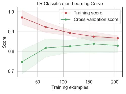
Let’s plot the LR Classification Learning Curve
skplt.estimators.plot_learning_curve(LogisticRegression(), X_train, y_train,
cv=7, shuffle=True, scoring=”accuracy”,
n_jobs=-1, figsize=(6,4), title_fontsize=”large”, text_fontsize=”large”,
title=”LR Classification Learning Curve”);
Let’s compare the classification scores
gb_classif = GradientBoostingClassifier()
gb_classif.fit(X_train, y_train)
gb_classif.score(X_test, y_test)
0.6557377049180327
rf_reg = RandomForestRegressor()
rf_reg.fit(X_train, y_train)
rf_reg.score(X_test, y_test)
0.2841965517241377
Let’s plot the final LR ROC Curve
log_reg=LogisticRegression()
log_reg.fit(X_train, y_train)
Y_test_probs = log_reg.predict_proba(X_test)
skplt.metrics.plot_roc_curve(y_test, Y_test_probs,
title=”LR ROC Curve”, figsize=(12,6));

Let’s plot again the final LR confusion matrix
cm = confusion_matrix(log_reg.predict(X_test),y_test)
target_names=[‘Low’,’High’]
cmn = cm.astype(‘float’) / cm.sum(axis=1)[:, np.newaxis]
fig, ax = plt.subplots(figsize=(10,10))
sns.heatmap(cmn, annot=True, fmt=’.2f’, xticklabels=target_names, yticklabels=target_names)
plt.ylabel(‘Actual’)
plt.xlabel(‘Predicted’)
plt.show(block=False)
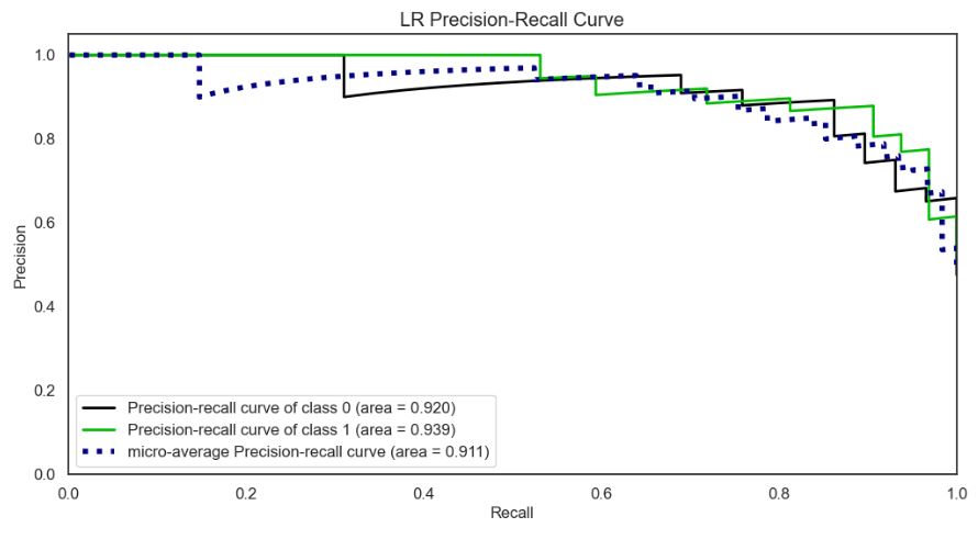
Let’s plot the LR Precision-Recall Curve
skplt.metrics.plot_precision_recall_curve(y_test, Y_test_probs,
title=”LR Precision-Recall Curve”, figsize=(12,6));
Let’s look at the KS Statistic plot
Y_probas = log_reg.predict_proba(X_test)
skplt.metrics.plot_ks_statistic(y_test, Y_probas, figsize=(10,6));

Let’s examine the Cumulative Gains Curve

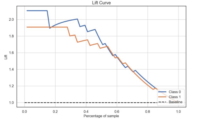
Let’s check the LR Lift Curve
skplt.metrics.plot_lift_curve(y_test, Y_probas, figsize=(10,6));
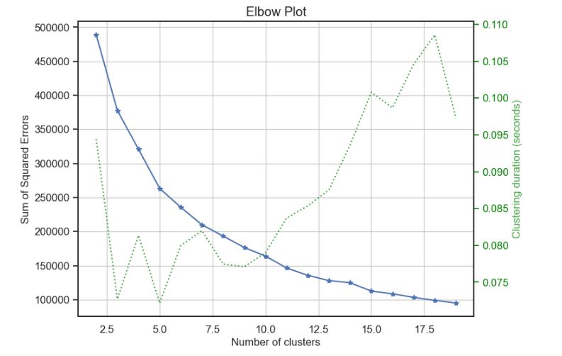
Let’s examine the Elbow Plot
skplt.cluster.plot_elbow_curve(KMeans(random_state=1),
X_train,
cluster_ranges=range(2, 20),
figsize=(8,6));
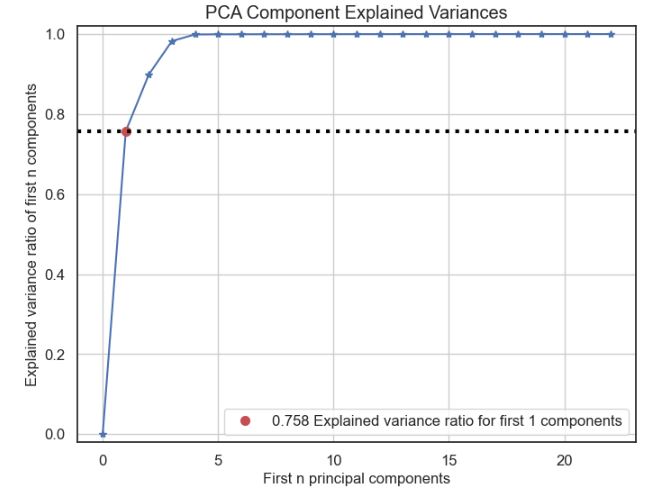
Let’s check PCA component explained variances
kmeans = KMeans(n_clusters=10, random_state=1)
kmeans.fit(X_train, y_train)
cluster_labels = kmeans.predict(X_test)
pca = PCA(random_state=1)
pca.fit(X_train)
skplt.decomposition.plot_pca_component_variance(pca, figsize=(8,6));
Let’s look at the yellowbricks threshold plot for LR
from sklearn.linear_model import LogisticRegression
from yellowbrick.classifier import DiscriminationThreshold
viz = DiscriminationThreshold(LogisticRegression(random_state=123),
classes=target_names,
cv=0.2,
fig=plt.figure(figsize=(9,6)))
viz.fit(X_train, y_train)
viz.score(X_test, y_test)
viz.show();

As an example of yellowbricks data visualization, let’s look at DecisionTreeClassifier
import pandas as pd
import numpy as np
import matplotlib.pyplot as plt
import sklearn
import yellowbrick
pd.set_option(“display.max_columns”, 35)
import warnings
warnings.filterwarnings(“ignore”)
from yellowbrick.classifier import ClassificationReport
from sklearn.tree import DecisionTreeClassifier
viz = ClassificationReport(DecisionTreeClassifier(random_state=123),
classes=target_names,
support=True,
fig=plt.figure(figsize=(8,6)))
viz.fit(X_train, y_train)
viz.score(X_test, y_test)
viz.show();

Let’ check the ROC curves for DecisionTreeClassifier
from yellowbrick.classifier import ROCAUC
viz = ROCAUC(DecisionTreeClassifier(random_state=123),
classes=target_names,
fig=plt.figure(figsize=(7,5)))
viz.fit(X_train, y_train)
viz.score(X_test, y_test)
viz.show();

Let’s plot the Precision-Recall Curve for DecisionTreeClassifier
from yellowbrick.classifier import PrecisionRecallCurve
viz = PrecisionRecallCurve(DecisionTreeClassifier(random_state=123),
classes=target_names,
ap_score=True,
iso_f1_curves=True,
fig=plt.figure(figsize=(7,5)))
viz.fit(X_train, y_train)
viz.score(X_test, y_test)
viz.show();

The same considerations apply to other ML algorithms mentioned above.
Summary
Part 1
- The ECG is a proven noninvasive test for predicting CVD. However, the ECG signal is prone to contamination by different kinds of noise. Such noise may cause deformation on the ECG heartbeat waveform, leading to cardiologists’ mislabeling or misinterpreting heartbeats.
- To address this problem, this paper proposes a robust and automated approach to analyse ECG signals using the Keras Sequential Autoencoder ANN. The autoencoder was trained to learn a representation of the input data that has a lower dimensionality than the original input. This is done by learning to reconstruct the input data from a compressed representation.
- Results show that losses.mae = 0.034331195 and the val_loss curve is

- It appears that the ANN training model can also handle noise associated with ECG-based time series signal, its achieved accuracy is extremely high and over fitting problems is solved in a robust and efficient manner.
Part 2
- In the second part of this paper, we present a ML-based heart attack prediction method in which the analysis of different risk factors and prediction for CVD is done using multiple supervised ML approaches.
- The data of heart disease symptoms has been collected from the UCI ML Repository and analysis has been performed on the data using ML methods. The focus has been on optimizing the prediction on the basis of different parameters.
- Logistic Regression and Ridge Classifier provided the best predictions among the 19 models. The AUC achieved with Ridge Classifier and Logistic Regression is .90. The prediction with ML models in identifying heart attack symptoms is highly efficient, especially with boosting algorithms. The prediction was done to evaluate accuracy, precision, recall, and area under the curve. ML models are being trained to perform optimized predictions.
- Results of in-depth performance QC for Logistic Regression (LR): the ROC curve of class 1 are = 0.93, LR classification learning curves – training score is 0.87 and cross-validation score is 0.83, precision-recall of class 1 area = 0.94, discrimination threshold value is 0.45, KS statistic is 0.768 at 0.159,
- According to the Random Forest Classifier, the top 3 most dominant features are oldpeak, Max_Heart_Rate, and age.
- PCA: the elbow plot yields 10 clusters, 0.758 explained variance ratio for the first 1 components.
- This study opens the doors to a new dimension for application of both autoencoders and supervised ML algorithms in predicting CVD by implementing hybrid models combined with various performance measures.
- This prediction can help clinically in analyzing the risk factors of the heart disease and ECG interpretation of the patient scenario. Optimizing the ML models provided promising results to predict early symptoms of CVD. It can further be optimized by working further on risk factors associated with this condition.
Explore More
- Using AI/ANN AUC>90% for Early Diagnosis of Cardiovascular Disease (CVD)
- DL-Assisted ECG/EKG Anomaly Detection using LSTM Autoencoder
- HealthTech ML/AI Use-Cases
- Heart Failure Prediction using Supervised ML/AI Technique
- ECG Early Warning System (EWS) in Terms of Time-Variant Deformations and Creep-Recovery Strain Tests
- ECG Early Warning System (EWS) in Terms of the Heart Stress-Strain Failure Curve
- AI-Based ECG Recognition – EOY ’22 Status
- HealthTech ML/AI Q3 ’22 Round-Up
- About


Make a one-time donation
Make a monthly donation
Make a yearly donation
Choose an amount
Or enter a custom amount
Your contribution is appreciated.
Your contribution is appreciated.
Your contribution is appreciated.

Leave a comment