
The goal of portfolio optimization is to build a stock portfolio that yields the maximum possible return while maintaining the amount of risk you’re willing to carry.
Referring to our previous case study, let’s invoke the stochastic optimization algorithm and the corresponding code to create an optimized portfolio by testing 10,000 combinations of the following 20 dividend growth stocks:
Table of Contents
Input Data Preparation
Let’s define the following input parameters
Tickers:
benchmark_ = [“^GSPC”]
portfolio_ = [‘V’, ‘O’, ‘HD’, ‘MO’, ‘WM’,’NEE’,’PEP’,’CAT’,’UNH’,’MCD’,’XOM’,’UNP’,’CNQ’,’LMT’,’BLK’,’AAPL’,’MSFT’,’SBUX’,’ASML’,
‘COST’]
Dates:
start_date_ = “2022-01-01”
end_date_ = “2023-03-03”
trade_days_per_year = 252
Stochastic Simulations:
number_of_scenarios = 10000
Risk %:
delta_risk = 0.1
Let’s set the working directory YOURPATH
import os
os.chdir(‘YOURPATH’)
os. getcwd()
and import the following libraries
import yfinance as yf
import pandas as pd
import numpy as np
import matplotlib.pyplot as plt
import squarify
import seaborn as sb
Let’s download our stock and benchmark data
return_vector = []
risk_vector = []
distrib_vector = []
df = yf.download(benchmark_, start=start_date_, end=end_date_)
df2 = yf.download(portfolio_, start=start_date_, end=end_date_)
Clean Rows with No Values on both Benchmark and Portfolio
df = df.dropna(axis=0)
df2 = df2.dropna(axis=0)
Matching the Days
df = df[df.index.isin(df2.index)]
[*********************100%***********************]  1 of 1 completed
[*********************100%***********************]  5 of 5 completed
df.tail()

df.shape
(292, 6)
df2.shape
(292, 120)
df.info()
<class 'pandas.core.frame.DataFrame'>
DatetimeIndex: 292 entries, 2022-01-03 to 2023-03-02
Data columns (total 6 columns):
 #   Column     Non-Null Count  Dtype
---  ------     --------------  -----
 0   Open       292 non-null    float64
 1   High       292 non-null    float64
 2   Low        292 non-null    float64
 3   Close      292 non-null    float64
 4   Adj Close  292 non-null    float64
 5   Volume     292 non-null    int64
dtypes: float64(5), int64(1)
memory usage: 16.0 KB
df2.columns
MultiIndex([('Adj Close', 'AAPL'),
            ('Adj Close', 'ASML'),
            ('Adj Close',  'BLK'),
            ('Adj Close',  'CAT'),
            ('Adj Close',  'CNQ'),
            ('Adj Close', 'COST'),
            ('Adj Close',   'HD'),
            ('Adj Close',  'LMT'),
            ('Adj Close',  'MCD'),
            ('Adj Close',   'MO'),
            ...
            (   'Volume', 'MSFT'),
            (   'Volume',  'NEE'),
            (   'Volume',    'O'),
            (   'Volume',  'PEP'),
            (   'Volume', 'SBUX'),
            (   'Volume',  'UNH'),
            (   'Volume',  'UNP'),
            (   'Volume',    'V'),
            (   'Volume',   'WM'),
            (   'Volume',  'XOM')],
           length=120)
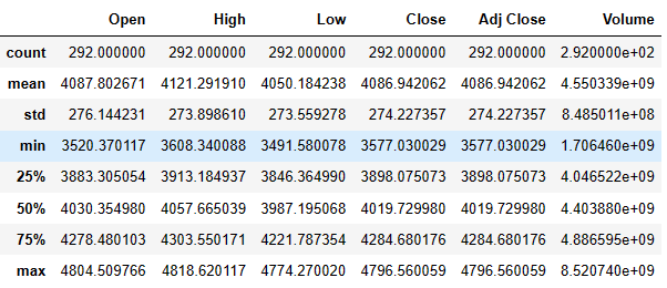
df.describe()
df2.describe().T

Portfolio/Benchmark Analysis
Analysis of Benchmark:
benchmark_vector = np.array(df[‘Close’])
Create our Daily Returns
benchmark_vector = np.diff(benchmark_vector)/benchmark_vector[1:]
Select or Final Return and Risk
benchmark_return = np.average(benchmark_vector)
benchmark_risk = np.std(benchmark_vector)
Add our Benchmark info to our lists
return_vector.append(benchmark_return)
risk_vector.append(benchmark_risk)
Analysis of Portfolio
portfolio_vector = np.array(df2[‘Close’])
Create a loop for the number of scenarios we want:
for i in range(number_of_scenarios):
#Create a random distribution that sums 1
# and is split by the number of stocks in the portfolio
random_distribution = np.random.dirichlet(np.ones(len(portfolio_)),size=1)
distrib_vector.append(random_distribution)
#Find the Closing Price for everyday of the portfolio
portfolio_matmul = np.matmul(random_distribution,portfolio_vector.T)

#Calculate the daily return
portfolio_matmul = np.diff(portfolio_matmul)/portfolio_matmul[:,1:]

#Select or Final Return and Risk
portfolio_return = np.average(portfolio_matmul, axis=1)
portfolio_risk = np.std(portfolio_matmul, axis=1)

#Add our Benchmark info to our lists
return_vector.append(portfolio_return[0])
risk_vector.append(portfolio_risk[0])
Create Risk Boundaries with the given delta_risk
min_risk = np.min(risk_vector)
max_risk = risk_vector[0]*(1+delta_risk)
risk_gap = [min_risk, max_risk]
Portfolio Return and Risk Couple
portfolio_array = np.column_stack((return_vector,risk_vector))[1:,]
Rule to create the best portfolio
If the criteria of minimum risk is satisfied then:
if np.where(((portfolio_array[:,1]<= max_risk)))[0].shape[0]>1:
min_risk_portfolio = np.where(((portfolio_array[:,1]<= max_risk)))[0]
best_portfolio_loc = portfolio_array[min_risk_portfolio]
max_loc = np.argmax(best_portfolio_loc[:,0])
best_portfolio = best_portfolio_loc[max_loc]
If the criteria of minimum risk is not satisfied then:
else:
min_risk_portfolio = np.where(((portfolio_array[:,1]== np.min(risk_vector[1:]))))[0]
best_portfolio_loc = portfolio_array[min_risk_portfolio]
max_loc = np.argmax(best_portfolio_loc[:,0])
best_portfolio = best_portfolio_loc[max_loc]
Let’s plot the summary of yearly portfolio average return vs standard deviation: portfolio scenarios, market proxy values, and best performer.
risk_gap = np.array(risk_gap)
best_portfolio[0] = np.array(best_portfolio[0])
x = np.array(risk_vector)
y = np.array(return_vector)*trade_days_per_year
fig, ax = plt.subplots(figsize=(20, 15))
plt.rc(‘axes’, titlesize=14) # Controls Axes Title
plt.rc(‘axes’, labelsize=14) # Controls Axes Labels
plt.rc(‘xtick’, labelsize=14) # Controls x Tick Labels
plt.rc(‘ytick’, labelsize=14) # Controls y Tick Labels
plt.rc(‘legend’, fontsize=14) # Controls Legend Font
plt.rc(‘figure’, titlesize=14) # Controls Figure Title
ax.scatter(x, y, alpha=0.5,
linewidths=0.1,
edgecolors=’black’, s=20,
label=’Portfolio Scenarios’
)
ax.scatter(x[0],
y[0],
color=’red’,
linewidths=1, s=180,
edgecolors=’black’,
label=’Market Proxy Values’)
ax.scatter(best_portfolio[1],
best_portfolio[0],
color=’green’,
linewidths=1, s=180,
edgecolors=’black’,
label=’Best Performer’)
ax.axvspan(min_risk,
max_risk,
color=’red’,
alpha=0.08,
label=’Accepted Risk Zone’)
ax.set_ylabel(“Yearly Portfolio Average Return (%)”,fontsize=14)
ax.set_xlabel(“Yearly Portfolio Standard Deviation”,fontsize=14)
ax.axhline(y=0, color=’black’,alpha=0.5)
ax = plt.gca()
ax.legend(loc=0)
vals = ax.get_yticks()
ax.set_yticklabels([‘{:,.2%}’.format(x) for x in vals])
plt.savefig(‘risk_optimizer2023.png’, dpi=300)

Output Data Visualization
let’s look at the Output Table of Distributions
portfolio_loc = np.where((portfolio_array[:,0]==(best_portfolio[0]/trade_days_per_year))&(portfolio_array[:,1]==(best_portfolio[1])))[0][0]
best_distribution = distrib_vector[portfolio_loc][0].tolist()
d = {“Stock Name”: portfolio_, “Stock % in Portfolio”: best_distribution}
output = pd.DataFrame(d)
output = output.sort_values(by=[“Stock % in Portfolio”],ascending=False)
output= output.style.format({“Stock % in Portfolio”: “{:.2%}”})
output

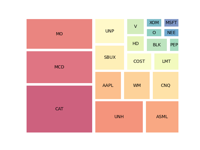
The can approximate this distribution by the squarify matrix proxy
episode_data =[20,14,13,10,7,5,5,5,5,5,3,3,2,2,2,1,1,1,1,1]
anime_names = [‘CAT’,’MCD’,’MO’,’UNH’,’ASML’,’AAPL’,’WM’,’CNQ’,’SBUX’,’UNP’,’COST’,’LMT’,’HD’,’V’,’BLK’,’PEP’,’O’,’XOM’,’NEE’,’MSFT’]
squarify.plot(episode_data, label=anime_names,color=sb.color_palette(“Spectral”,
len(episode_data)),alpha=.7,pad=2)
plt.axis(“off”)
plt.savefig(‘squarify20stocks.png’)
Summary
In this post, we have invoked the stochastic portfolio optimization algorithm to create a balanced portfolio of 20 dividend growth stocks suggested by @DrDividend47. Results allow us to spread our investment capital across a variety of assets. As a result, we can balance those assets in order to attain our desired min (risk) and max(reward) outcome whilst outperforming the benchmark index ^GSPC.
Explore More
- Bear vs. Bull Portfolio Risk/Return Optimization QC Analysis
- Risk/Return POA – Dr. Dividend’s Positions
- Portfolio Optimization Risk/Return QC – Positions of Humble Div vs Dividend Glenn
- Risk/Return QC via Portfolio Optimization – Current Positions of The Dividend Breeder
- Stock Portfolio Risk/Return Optimization


Make a one-time donation
Make a monthly donation
Make a yearly donation
Choose an amount
Or enter a custom amount
Your contribution is appreciated.
Your contribution is appreciated.
Your contribution is appreciated.
DonateDonate monthlyDonate yearly
Leave a comment