
As Goethe once said, “Life is too short to drink bad wine.”
Predicting wine quality using ML/AI techniques is becoming increasingly popular today. ML models can tell us exactly what makes a good quality wine.
Today we will compare the key multi-label classifiers used for wine quality prediction in ML algorithms. Our specific goals are as follows:
1. To experiment with different classification methods to see which yields the highest accuracy;
2. To determine which features are the most indicative of a good quality wine.
Our end-to-end Python workflow consist of the following steps:
- Input Data Preparation/Editing
- Exploratory Data Analysis (EDA)
- Data Pre-Processing
- Data Manipulation/Transformation
- Feature Engineering (Selection/Extraction)
- Predictive Training/Resting Modelling
- ML QC Performance Report
Description of 12 Attributes
There are the following 12 features including the target parameter:
- fixed acidity (tartaric acid – g / dm^3) : most acids involved with wine or fixed or nonvolatile (do not evaporate readily)
- volatile acidity (acetic acid – g / dm^3) : the amount of acetic acid in wine, which at too high of levels can lead to an unpleasant, vinegar taste
- citric acid (g / dm^3) : found in small quantities, citric acid can add ‘freshness’ and flavor to wines
- residual sugar (g / dm^3) : the amount of sugar remaining after fermentation stops, it’s rare to find wines with less than 1 gram/liter and wines with greater than 45 grams/liter are considered sweet
- chlorides (sodium chloride – g / dm^3) : the amount of salt in the wine
- free sulfur dioxide (mg / dm^3) : the free form of SO2 exists in equilibrium between molecular SO2 (as a dissolved gas) and bisulfite ion; it prevents microbial growth and the oxidation of wine
- total sulfur dioxide (mg / dm^3) : amount of free and bound forms of S02; in low concentrations, SO2 is mostly undetectable in wine, but at free SO2 concentrations over 50 ppm, SO2 becomes evident in the nose and taste of wine
- density (g / cm^3) : the density of water is close to that of water depending on the percent alcohol and sugar content
- pH: describes how acidic or basic a wine is on a scale from 0 (very acidic) to 14 (very basic); most wines are between 3-4 on the pH scale
- sulphates (potassium sulphate – g / dm3) : a wine additive which can contribute to sulfur dioxide gas (S02) levels, which acts as an antimicrobial and antioxidant
- alcohol (% by volume) : the percentage of wine alcohol content
- quality (score between 0 and 10)
Import Libraries
Let’s set the working directory YOURPATH
import os
os.chdir(‘YOURPATH’)
os. getcwd()
and import the basic libraries
import math
import scipy
import numpy as np
import pandas as pd
import seaborn as sns
from tqdm import tqdm
from sklearn import tree
from scipy.stats import randint
from scipy.stats import loguniform
from IPython.display import display
from sklearn.decomposition import PCA
from imblearn.over_sampling import SMOTE
from sklearn.feature_selection import RFE
from sklearn.preprocessing import OneHotEncoder
from sklearn.preprocessing import StandardScaler
from sklearn.model_selection import train_test_split
from statsmodels.stats.outliers_influence import variance_inflation_factor
from sklearn.model_selection import RandomizedSearchCV
from sklearn.model_selection import RepeatedStratifiedKFold
from sklearn.svm import SVC
from xgboost import XGBClassifier
from sklearn.naive_bayes import BernoulliNB
from sklearn.tree import DecisionTreeClassifier
from sklearn.ensemble import RandomForestClassifier
from sklearn.linear_model import LogisticRegression
from sklearn.neighbors import KNeighborsClassifier
from sklearn.ensemble import GradientBoostingClassifier
from sklearn.linear_model import LinearRegression
from sklearn.preprocessing import PolynomialFeatures
from scikitplot.metrics import plot_roc_curve as auc_roc
from sklearn.metrics import accuracy_score, confusion_matrix, classification_report, \
f1_score, roc_auc_score, roc_curve, precision_score, recall_score
import matplotlib.pyplot as plt
plt.rcParams[‘figure.figsize’] = [10,6]
import warnings
warnings.filterwarnings(‘ignore’)
pd.set_option(‘display.max_columns’, 50)
Input Dataset
Importing the input Kaggle dataset
df = pd.read_csv(‘WineQT.csv’)
Let’s define the target variable and model features
target = ‘quality’
labels = [‘Quality-3′,’Quality-4′,’Quality-5′,’Quality-6′,’Quality-7′,’Quality-8’]
features = [i for i in df.columns.values if i not in [target]]
original_df = df.copy(deep=True)
display(df.head())
print(‘\n\033[1mInference:\033[0m The Dataset consists of {} features & {} samples.’.format(df.shape[1], df.shape[0]))

Inference: The Dataset consists of 13 features & 1143 samples.
Checking the dtypes of all the columns
df.info()
<class 'pandas.core.frame.DataFrame'>
RangeIndex: 1143 entries, 0 to 1142
Data columns (total 13 columns):
 #   Column                Non-Null Count  Dtype
---  ------                --------------  -----
 0   fixed acidity         1143 non-null   float64
 1   volatile acidity      1143 non-null   float64
 2   citric acid           1143 non-null   float64
 3   residual sugar        1143 non-null   float64
 4   chlorides             1143 non-null   float64
 5   free sulfur dioxide   1143 non-null   float64
 6   total sulfur dioxide  1143 non-null   float64
 7   density               1143 non-null   float64
 8   pH                    1143 non-null   float64
 9   sulphates             1143 non-null   float64
 10  alcohol               1143 non-null   float64
 11  quality               1143 non-null   int64
 12  Id                    1143 non-null   int64
dtypes: float64(11), int64(2)
memory usage: 116.2 KB
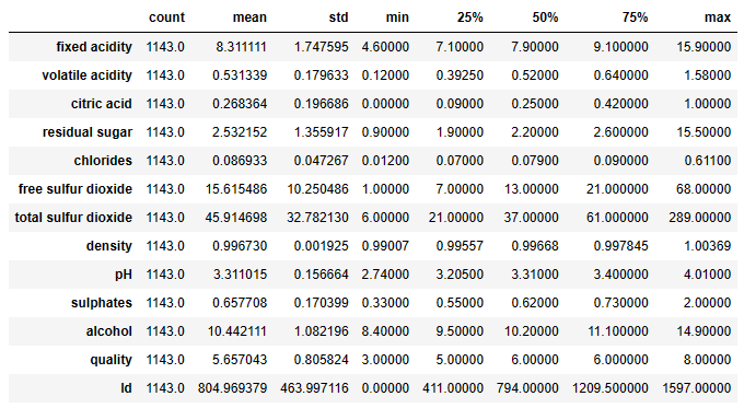
Run the descriptive statistics
df.describe().T
Checking the number of feature unique values
df.nunique().sort_values()
quality                    6
free sulfur dioxide       53
alcohol                   61
citric acid               77
residual sugar            80
pH                        87
sulphates                 89
fixed acidity             91
chlorides                131
volatile acidity         135
total sulfur dioxide     138
density                  388
Id                      1143
dtype: int64
Checking the number of unique rows in each feature
nu = df[features].nunique().sort_values()
nf = []; cf = []; nnf = 0; ncf = 0; #numerical & categorical features
for i in range(df[features].shape[1]):
if nu.values[i]<=7:cf.append(nu.index[i])
else: nf.append(nu.index[i])
print(‘\n\033[1mInference:\033[0m The Dataset has {} numerical & {} categorical features.’.format(len(nf),len(cf)))
Inference: The Dataset has 12 numerical & 0 categorical features.
Exploratory Data Analysis (EDA)
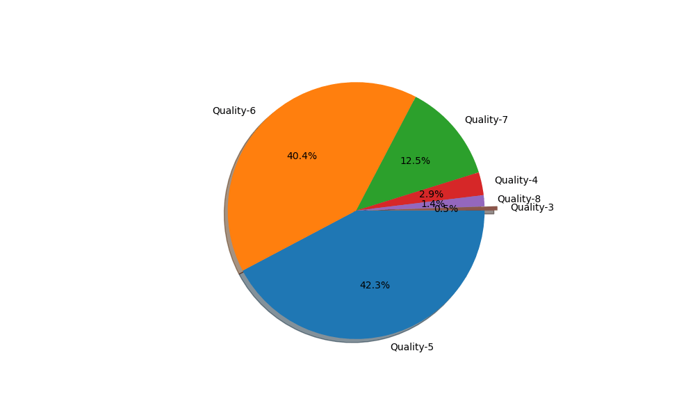
Let us first analyze the distribution of the target variable
MAP={}
for e, i in enumerate(sorted(df[target].unique())):
MAP[i]=labels[e]
df1 = df.copy()
df1[target]=df1[target].map(MAP)
explode=np.zeros(len(labels))
explode[-1]=0.1
print(‘\033[1mTarget Variable Distribution’.center(55))
plt.pie(df1[target].value_counts(), labels=df1[target].value_counts().index, counterclock=False, shadow=True,
explode=explode, autopct=’%1.1f%%’, radius=1, startangle=0)
plt.savefig(“winetargetvariable.png”)
Target Variable Distribution:
Understanding the feature set
print(‘\033[1mFeatures Distribution’.center(100))
nf = [i for i in features if i not in cf]
n=4
plt.figure(figsize=[15,2.5*math.ceil(len(features)/n)])
for c in range(len(nf)):
plt.subplot(math.ceil(len(features)/n),n,c+1)
sns.distplot(df[nf[c]])
plt.tight_layout()
plt.show()
plt.figure(figsize=[15,2.5*math.ceil(len(features)/n)])
for c in range(len(nf)):
plt.subplot(math.ceil(len(features)/n),n,c+1)
df.boxplot(nf[c])
plt.tight_layout()
plt.savefig(“winefeaturedistribution.png”)


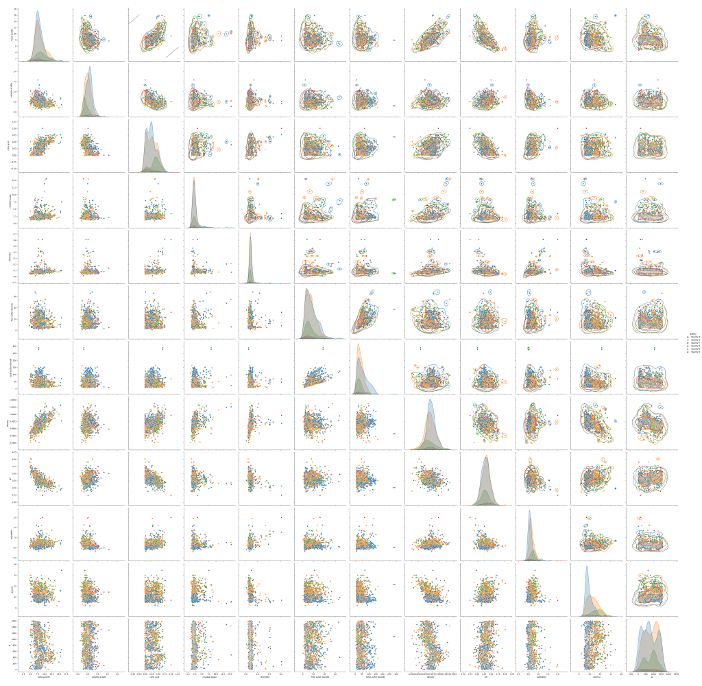
Let’s look at the pair plots
g=sns.pairplot(df1, hue=target, size=4)
g.map_upper(sns.kdeplot, levels=1, color=”.2″)
plt.savefig(“winepairplot.png”)
Data Pre-Processing
Removal of Duplicate rows if any
counter = 0
r,c = original_df.shape
df1 = df.copy()
df1.drop_duplicates(inplace=True)
df1.reset_index(drop=True,inplace=True)
if df1.shape==(r,c):
print(‘\n\033[1mInference:\033[0m The dataset doesn\’t have any duplicates’)
else:
print(f’\n\033[1mInference:\033[0m Number of duplicates dropped —> {r-df1.shape[0]}’)
Inference: The dataset doesn't have any duplicates
Check for Null elements
nvc = pd.DataFrame(df1.isnull().sum().sort_values(), columns=[‘Total Null Values’])
nvc[‘Percentage’] = round(nvc[‘Total Null Values’]/df1.shape[0],3)*100
print(nvc)
Total Null Values  Percentage
fixed acidity                         0         0.0
volatile acidity                      0         0.0
citric acid                           0         0.0
residual sugar                        0         0.0
chlorides                             0         0.0
free sulfur dioxide                   0         0.0
total sulfur dioxide                  0         0.0
density                               0         0.0
pH                                    0         0.0
sulphates                             0         0.0
alcohol                               0         0.0
quality                               0         0.0
Id                                    0         0.0
Removal of outliers:
df4 = df3.copy()
for i in [i for i in df4.columns]:
if df4[i].nunique()>=12:
Q1 = df4[i].quantile(0.06)
Q3 = df4[i].quantile(0.94)
IQR = Q3 – Q1
df4 = df4[df4[i] <= (Q3+(1.5IQR))] df4 = df4[df4[i] >= (Q1-(1.5IQR))]
df4 = df4.reset_index(drop=True)
display(df4.head())
print(‘\n\033[1mInference:\033[0m Before removal of outliers, The dataset had {} samples.’.format(df1.shape[0]))
print(‘\033[1mInference:\033[0m After removal of outliers, The dataset now has {} samples.’.format(df4.shape[0]))
Inference: Before removal of outliers, The dataset had 1143 samples.
Inference: After removal of outliers, The dataset now has 1106 samples.
Fixing the imbalance using SMOTE
df5 = df4.copy()
print(‘Original class distribution:’)
print(df5[target].value_counts())
xf = df5.columns
X = df5.drop([target],axis=1)
Y = df5[target]
smote = SMOTE()
X, Y = smote.fit_resample(X, Y)
df5 = pd.DataFrame(X, columns=xf)
df5[target] = Y
print(‘\nClass distribution after applying SMOTE Technique:’,)
print(Y.value_counts())
Original class distribution:
5    467
6    445
7    140
4     32
8     16
3      6
Name: quality, dtype: int64

Class distribution after applying SMOTE Technique:
5    467
6    467
7    467
4    467
8    467
3    467
Name: quality, dtype: int64
Final Dataset size after performing Pre-Processing
df = df5.copy()
plt.title(‘Final Dataset Samples’)
plt.pie([df.shape[0], original_df.shape[0]-df4.shape[0], df5.shape[0]-df4.shape[0]], radius = 1, shadow=True,
labels=[‘Retained’,’Dropped’,’Augmented’], counterclock=False, autopct=’%1.1f%%’, pctdistance=0.9, explode=[0,0,0])
plt.pie([df.shape[0]], labels=[‘100%’], labeldistance=-0, radius=0.78, shadow=True, colors=[‘powderblue’])
plt.savefig(“winesmot.png”)
print(‘\n\033[1mInference:\033[0mThe final dataset after cleanup has {} samples & {} columns.’.format(df.shape[0], df.shape[1]))
Inference:The final dataset after cleanup has 2802 samples & 13 columns.

Data Preparation
Splitting the data intro training & testing sets
df = df5.copy()
X = df.drop([target],axis=1)
Y = df[target]
Train_X, Test_X, Train_Y, Test_Y = train_test_split(X, Y, train_size=0.8, test_size=0.2, random_state=0)
print(‘Original set —> ‘,X.shape,Y.shape,’\nTraining set —> ‘,Train_X.shape,Train_Y.shape,’\nTesting set —> ‘, Test_X.shape,”, Test_Y.shape)
Original set  --->  (2802, 12) (2802,)
Training set  --->  (2241, 12) (2241,)
Testing set   --->  (561, 12)  (561,)
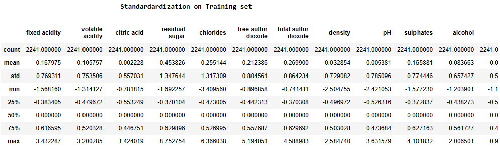
Feature Scaling (Standardization):
from sklearn.preprocessing import StandardScaler,RobustScaler,MinMaxScaler
std = RobustScaler()
print(‘\033[1mStandardardization on Training set’.center(100))
Train_X_std = std.fit_transform(Train_X)
Train_X_std = pd.DataFrame(Train_X_std, columns=X.columns)
display(Train_X_std.describe())
print(‘\n’,’\033[1mStandardardization on Testing set’.center(100))
Test_X_std = std.transform(Test_X)
Test_X_std = pd.DataFrame(Test_X_std, columns=X.columns)
display(Test_X_std.describe())
Feature Engineering (FE)
Checking the correlation matrix
features = df.columns
plt.figure(figsize=[12,10])
plt.title(‘Features Correlation-Plot’)
sns.heatmap(df[features].corr(), vmin=-1, vmax=1, center=0, annot=True)
plt.savefig(“winecorrmatrix.png”)

Let’s calculate the VIFs to remove multicollinearity
DROP=[]; scores1=[]; scores2=[]; scores3=[]
scores1.append(f1_score(Test_Y,LogisticRegression().fit(Train_X_std.drop(DROP,axis=1), Train_Y).predict(Test_X_std.drop(DROP,axis=1)),average=’weighted’)100) scores2.append(f1_score(Test_Y,RandomForestClassifier().fit(Train_X_std.drop(DROP,axis=1), Train_Y).predict(Test_X_std.drop(DROP,axis=1)),average=’weighted’)100)
scores3.append(f1_score(Test_Y,DecisionTreeClassifier().fit(Train_X_std.drop(DROP,axis=1), Train_Y).predict(Test_X_std.drop(DROP,axis=1)),average=’weighted’)*100)
for i in tqdm(range(len(X.columns.values)-1)):
vif = pd.DataFrame()
Xs = X.drop(DROP,axis=1)
vif[‘Features’] = Xs.columns
vif[‘VIF’] = [variance_inflation_factor(Xs.values, i) for i in range(Xs.shape[1])]
vif[‘VIF’] = round(vif[‘VIF’], 2)
vif = vif.sort_values(by = “VIF”, ascending = False)
vif.reset_index(drop=True, inplace=True)
DROP.append(vif.Features[0])
if vif.VIF[0]>1:
scores1.append(f1_score(Test_Y,LogisticRegression().fit(Train_X_std.drop(DROP,axis=1), Train_Y).predict(Test_X_std.drop(DROP,axis=1)),average=’weighted’)100) scores2.append(f1_score(Test_Y,RandomForestClassifier().fit(Train_X_std.drop(DROP,axis=1), Train_Y).predict(Test_X_std.drop(DROP,axis=1)),average=’weighted’)100)
scores3.append(f1_score(Test_Y,DecisionTreeClassifier().fit(Train_X_std.drop(DROP,axis=1), Train_Y).predict(Test_X_std.drop(DROP,axis=1)),average=’weighted’)*100)
plt.plot(scores1, label=’LR’)
plt.plot(scores2, label=’RF’)
plt.plot(scores3, label=’DT’)
plt.legend()
plt.grid()
plt.savefig(“winemanualvif.png”)

Let’s apply the automated method – RFE
Applying Recursive Feature Elimination
LR = LogisticRegression()#.fit(Train_X_std, Train_Y)
scores1=[]; scores2=[]; scores3=[]
scores1.append(f1_score(Test_Y,LogisticRegression(solver=’liblinear’).fit(Train_X_std, Train_Y).predict(Test_X_std),average=’weighted’)100) scores2.append(f1_score(Test_Y,RandomForestClassifier().fit(Train_X_std, Train_Y).predict(Test_X_std),average=’weighted’)100)
scores3.append(f1_score(Test_Y,DecisionTreeClassifier().fit(Train_X_std, Train_Y).predict(Test_X_std),average=’weighted’)*100)
for i in tqdm(range(len(X.columns.values))):
rfe = RFE(LR,n_features_to_select=len(Train_X_std.columns)-i)
rfe = rfe.fit(Train_X_std, Train_Y)
scores1.append(f1_score(Test_Y,LogisticRegression(solver=’liblinear’).fit(Train_X_std[Train_X_std.columns[rfe.support_]], Train_Y).predict(Test_X_std[Train_X_std.columns[rfe.support_]]),average=’weighted’)100) scores2.append(f1_score(Test_Y,RandomForestClassifier().fit(Train_X_std[Train_X_std.columns[rfe.support_]], Train_Y).predict(Test_X_std[Train_X_std.columns[rfe.support_]]),average=’weighted’)100)
scores3.append(f1_score(Test_Y,DecisionTreeClassifier().fit(Train_X_std[Train_X_std.columns[rfe.support_]], Train_Y).predict(Test_X_std[Train_X_std.columns[rfe.support_]]),average=’weighted’)*100)
plt.plot(scores1, label=’LR’)
plt.plot(scores2, label=’RF’)
plt.plot(scores3, label=’DT’)
plt.legend()
plt.grid()
plt.savefig(“wineautomatedrfe.png”)
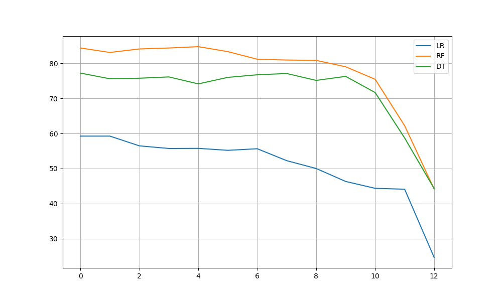
Let’s invoke PCA
from sklearn.decomposition import PCA
pca = PCA().fit(Train_X_std)
fig, ax = plt.subplots(figsize=(14,6))
x_values = range(1, pca.n_components_+1)
ax.bar(x_values, pca.explained_variance_ratio_, lw=2, label=’Explained Variance’)
ax.plot(x_values, np.cumsum(pca.explained_variance_ratio_), lw=2, label=’Cumulative Explained Variance’, color=’red’)
plt.plot([0,pca.n_components_+1],[0.90,0.90],’g–‘)
plt.plot([7,7],[0,1], ‘g–‘)
ax.set_title(‘Explained variance of components’)
ax.set_xlabel(‘Principal Component’)
ax.set_ylabel(‘Explained Variance’)
plt.grid()
plt.legend()
plt.savefig(“winepcavariance.png”)
Applying PCA Transformations
scores1=[]; scores2=[]; scores3=[]
for i in tqdm(range(len(X.columns.values))):
pca = PCA(n_components=Train_X_std.shape[1]-i)
Train_X_std_pca = pca.fit_transform(Train_X_std)
Train_X_std_pca = pd.DataFrame(Train_X_std_pca)

Test_X_std_pca = pca.transform(Test_X_std)

Test_X_std_pca = pd.DataFrame(Test_X_std_pca)

scores1.append(f1_score(Test_Y,LogisticRegression(solver='liblinear').fit(Train_X_std_pca, Train_Y).predict(Test_X_std_pca),average='weighted')*100)
scores2.append(f1_score(Test_Y,RandomForestClassifier().fit(Train_X_std_pca, Train_Y).predict(Test_X_std_pca),average='weighted')*100)
scores3.append(f1_score(Test_Y,DecisionTreeClassifier().fit(Train_X_std_pca, Train_Y).predict(Test_X_std_pca),average='weighted')*100)
plt.plot(scores1, label=’LR’)
plt.plot(scores2, label=’RF’)
plt.plot(scores3, label=’DT’)
plt.legend()
plt.grid()
plt.savefig(“winepcatransform.png”)

Finalising the shortlisted features
rfe = RFE(LR,n_features_to_select=len(Train_X_std.columns))
rfe = rfe.fit(Train_X_std, Train_Y)
print(f1_score(Test_Y,LogisticRegression().fit(Train_X_std[Train_X_std.columns[rfe.support_]], Train_Y).predict(Test_X_std[Train_X_std.columns[rfe.support_]]),average=’weighted’)100) print(f1_score(Test_Y,RandomForestClassifier().fit(Train_X_std[Train_X_std.columns[rfe.support_]], Train_Y).predict(Test_X_std[Train_X_std.columns[rfe.support_]]),average=’weighted’)100)
print(f1_score(Test_Y,DecisionTreeClassifier().fit(Train_X_std[Train_X_std.columns[rfe.support_]], Train_Y).predict(Test_X_std[Train_X_std.columns[rfe.support_]]),average=’weighted’)*100)
print(Train_X_std.shape)
print(Test_X_std.shape)
61.18536559387585
83.58268375137607
75.9904516868097
(2241, 12)
(561, 12)
Train/Test Models
Let’s initialize the 7×5 table of ML results
Evaluation_Results = pd.DataFrame(np.zeros((7,5)), columns=[‘Accuracy’, ‘Precision’,’Recall’,’F1-score’,’AUC-ROC score’])
Evaluation_Results.index=[‘Logistic Regression (LR)’,’Decision Tree Classifier (DT)’,’Random Forest Classifier (RF)’,’Naïve Bayes Classifier (NB)’,
‘Support Vector Machine (SVM)’,’K Nearest Neighbours (KNN)’, ‘Gradient Boosting (GB)’]
Let’s define the Classification Summary Functions
def Classification_Summary(pred,pred_prob,i):
Evaluation_Results.iloc[i][‘Accuracy’]=round(accuracy_score(Test_Y, pred)*100 Evaluation_Results.iloc[i][‘Precision’]=round(precision_score(Test_Y, pred, average=’weighted’)*100
Evaluation_Results.iloc[i][‘Recall’]=round(recall_score(Test_Y, pred, average=’weighted’)*100
Evaluation_Results.iloc[i][‘F1-score’]=round(f1_score(Test_Y, pred, average=’weighted’)*100
Evaluation_Results.iloc[i][‘AUC-ROC score’]=round(roc_auc_score(Test_Y, pred_prob, multi_class=’ovr’)*100
print(‘{}{}\033[1m Evaluating {} \033[0m{}{}\n’.format(‘<‘3,’-35,Evaluation_Results.index[i], ‘-‘35,’>’3))
print(‘Accuracy = {}%’.format(round(accuracy_score(Test_Y, pred)*100))
print(‘F1 Score = {}%’.format(round(f1_score(Test_Y, pred, average=’weighted’)*100))
print(‘\n \033[1mConfusion Matrix:\033[0m\n’,confusion_matrix(Test_Y, pred))
print(‘\n\033[1mClassification Report:\033[0m\n’,classification_report(Test_Y, pred))
auc_roc(Test_Y, pred_prob, curves=[‘each_class’])
plt.show()
Visualising Function
def AUC_ROC_plot(Test_Y, pred):
ref = [0 for _ in range(len(Test_Y))]
ref_auc = roc_auc_score(Test_Y, ref)
lr_auc = roc_auc_score(Test_Y, pred)
ns_fpr, ns_tpr, _ = roc_curve(Test_Y, ref)
lr_fpr, lr_tpr, _ = roc_curve(Test_Y, pred)

plt.plot(ns_fpr, ns_tpr, linestyle='--')
plt.plot(lr_fpr, lr_tpr, marker='.', label='AUC = {}'.format(round(roc_auc_score(Test_Y, pred)*100,2)))
plt.xlabel('False Positive Rate')
plt.ylabel('True Positive Rate')
plt.legend()
plt.show()
Building Logistic Regression (LR) Classifier
LR_model = LogisticRegression(solver=’liblinear’)
space = dict()
space[‘solver’] = [‘newton-cg’, ‘lbfgs’, ‘liblinear’]
space[‘penalty’] = [‘l2′] #’none’, ‘l1’, ‘l2’, ‘elasticnet’
space[‘C’] = loguniform(1e-5, 100)
cv = RepeatedStratifiedKFold(n_splits=10, n_repeats=3, random_state=1)
LR = LR_model.fit(Train_X_std, Train_Y)#.best_estimator_
pred = LR.predict(Test_X_std)
pred_prob = LR.predict_proba(Test_X_std)
Classification_Summary(pred,pred_prob,0)
print(‘\n\033[1mInterpreting the Output of Logistic Regression:\n\033[0m’)
print(‘intercept ‘, LR.intercept_[0])
print(‘classes’, LR.classes_)
display(pd.DataFrame({‘coeff’: LR.coef_[0]}, index=Train_X_std.columns))
<<<----------------------------------- Evaluating Logistic Regression (LR) ----------------------------------->>>

Accuracy = 61.5%
F1 Score = 59.199999999999996%

 Confusion Matrix:
 [[89  0  0  0  0  0]
 [ 8 46 13  7  7  0]
 [10 19 50  9  5  4]
 [ 4 14 29 29 16 10]
 [ 1  3  2 15 42 32]
 [ 0  0  0  0  8 89]]

Classification Report:
               precision    recall  f1-score   support

           3       0.79      1.00      0.89        89
           4       0.56      0.57      0.56        81
           5       0.53      0.52      0.52        97
           6       0.48      0.28      0.36       102
           7       0.54      0.44      0.49        95
           8       0.66      0.92      0.77        97

    accuracy                           0.61       561
   macro avg       0.59      0.62      0.60       561
weighted avg       0.59      0.61      0.59       561

Interpreting the Output of Logistic Regression:

intercept  -5.862113339389565
classes [3 4 5 6 7 8]

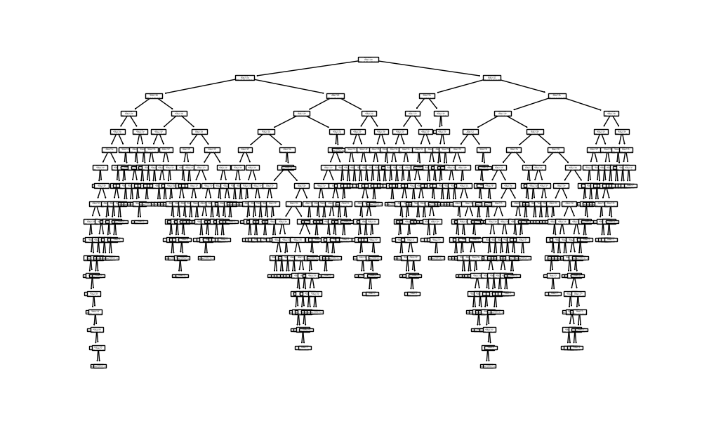
Building Decision Tree Classifier (DTC)
DT_model = DecisionTreeClassifier()
param_dist = {“max_depth”: [3, None],
“max_features”: randint(1, len(features)-1),
“min_samples_leaf”: randint(1, len(features)-1),
“criterion”: [“gini”, “entropy”]}
cv = RepeatedStratifiedKFold(n_splits=10, n_repeats=3, random_state=1)
RCV = RandomizedSearchCV(DT_model, param_dist, n_iter=50, scoring=’f1_weighted’, n_jobs=-1, cv=5, random_state=1)
DT = RCV.fit(Train_X_std, Train_Y).best_estimator_
pred = DT.predict(Test_X_std)
pred_prob = DT.predict_proba(Test_X_std)
Classification_Summary(pred,pred_prob,1)
print(‘\n\033[1mInterpreting the output of Decision Tree:\n\033[0m’)
tree.plot_tree(DT)
plt.savefig(“winedecisiontree.png”)
<<<----------------------------------- Evaluating Decision Tree Classifier (DT) ----------------------------------->>>

Accuracy = 75.6%
F1 Score = 75.0%

 Confusion Matrix:
 [[87  0  2  0  0  0]
 [ 1 72  5  3  0  0]
 [ 3 12 50 30  1  1]
 [ 1  8 24 51 16  2]
 [ 0  1  8 10 70  6]
 [ 0  0  0  0  3 94]]

Classification Report:
               precision    recall  f1-score   support

           3       0.95      0.98      0.96        89
           4       0.77      0.89      0.83        81
           5       0.56      0.52      0.54        97
           6       0.54      0.50      0.52       102
           7       0.78      0.74      0.76        95
           8       0.91      0.97      0.94        97

    accuracy                           0.76       561
   macro avg       0.75      0.76      0.76       561
weighted avg       0.75      0.76      0.75       561

Interpreting the output of Decision Tree:
Building Random-Forest Classifier (RFC)
RF_model = RandomForestClassifier()
param_dist={‘bootstrap’: [True, False],
‘max_depth’: [10, 20, 50, 100, None],
‘max_features’: [‘auto’, ‘sqrt’],
‘min_samples_leaf’: [1, 2, 4],
‘min_samples_split’: [2, 5, 10],
‘n_estimators’: [50, 100]}
cv = RepeatedStratifiedKFold(n_splits=10, n_repeats=3, random_state=1)
RCV = RandomizedSearchCV(RF_model, param_dist, n_iter=50, scoring=’f1_weighted’, n_jobs=-1, cv=5, random_state=1)
RF = RCV.fit(Train_X_std, Train_Y).best_estimator_
pred = RF.predict(Test_X_std)
pred_prob = RF.predict_proba(Test_X_std)
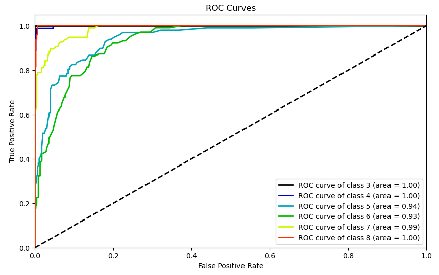
Classification_Summary(pred,pred_prob,2)
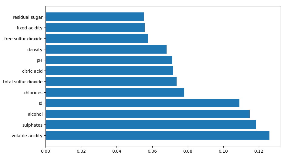
print(‘\n\033[1mInterpreting the output of Random Forest:\n\033[0m’)
rfi=pd.Series(RF.feature_importances_, index=Train_X_std.columns).sort_values(ascending=False)
plt.barh(rfi.index,rfi.values)
<<<----------------------------------- Evaluating Random Forest Classifier (RF) ----------------------------------->>>

Accuracy = 86.5%
F1 Score = 86.2%

 Confusion Matrix:
 [[89  0  0  0  0  0]
 [ 0 79  2  0  0  0]
 [ 0  2 73 17  4  1]
 [ 0  2 22 66  9  3]
 [ 0  0  0 11 81  3]
 [ 0  0  0  0  0 97]]

Classification Report:
               precision    recall  f1-score   support

           3       1.00      1.00      1.00        89
           4       0.95      0.98      0.96        81
           5       0.75      0.75      0.75        97
           6       0.70      0.65      0.67       102
           7       0.86      0.85      0.86        95
           8       0.93      1.00      0.97        97

    accuracy                           0.86       561
   macro avg       0.87      0.87      0.87       561
weighted avg       0.86      0.86      0.86       561
Interpreting the output of Random Forest:
Building Naive Bayes Classifier (NBC)
NB_model = BernoulliNB()
params = {‘alpha’: [0.01, 0.1, 0.5, 1.0, 10.0]}
cv = RepeatedStratifiedKFold(n_splits=10, n_repeats=3, random_state=1)
RCV = RandomizedSearchCV(NB_model, params, n_iter=50, scoring=’f1_weighted’, n_jobs=-1, cv=5, random_state=1)
NB = RCV.fit(Train_X_std, Train_Y).best_estimator_
pred = NB.predict(Test_X_std)
pred_prob = NB.predict_proba(Test_X_std)
Classification_Summary(pred,pred_prob,3)
<<<----------------------------------- Evaluating Naïve Bayes Classifier (NB) ----------------------------------->>>

Accuracy = 46.9%
F1 Score = 45.0%

 Confusion Matrix:
 [[66 14  9  0  0  0]
 [16 41 15  6  3  0]
 [19 17 46  6  5  4]
 [11 15 24 16 15 21]
 [ 0  4  2 21 33 35]
 [ 0  9  0  1 26 61]]

Classification Report:
               precision    recall  f1-score   support

           3       0.59      0.74      0.66        89
           4       0.41      0.51      0.45        81
           5       0.48      0.47      0.48        97
           6       0.32      0.16      0.21       102
           7       0.40      0.35      0.37        95
           8       0.50      0.63      0.56        97

    accuracy                           0.47       561
   macro avg       0.45      0.48      0.45       561
weighted avg       0.45      0.47      0.45       561

Building Support Vector Machine Classifier (SVMC)
SVM_model = SVC(probability=True).fit(Train_X_std, Train_Y)
svm_param = {“C”: [.01, .1, 1, 5, 10, 100],
“gamma”: [.01, .1, 1, 5, 10, 100],
“kernel”: [“rbf”],
“random_state”: [1]}
cv = RepeatedStratifiedKFold(n_splits=10, n_repeats=3, random_state=1)
SVM = SVM_model.fit(Train_X_std, Train_Y)#.best_estimator_
pred = SVM.predict(Test_X_std)
pred_prob = SVM.predict_proba(Test_X_std)
Classification_Summary(pred,pred_prob,4)
<<<----------------------------------- Evaluating Support Vector Machine (SVM) ----------------------------------->>>

Accuracy = 76.5%
F1 Score = 75.3%

 Confusion Matrix:
 [[89  0  0  0  0  0]
 [ 0 76  3  2  0  0]
 [ 3 15 59 15  4  1]
 [ 3  7 30 43 15  4]
 [ 0  0  0 17 67 11]
 [ 0  0  0  0  2 95]]

Classification Report:
               precision    recall  f1-score   support

           3       0.94      1.00      0.97        89
           4       0.78      0.94      0.85        81
           5       0.64      0.61      0.62        97
           6       0.56      0.42      0.48       102
           7       0.76      0.71      0.73        95
           8       0.86      0.98      0.91        97

    accuracy                           0.76       561
   macro avg       0.75      0.78      0.76       561
weighted avg       0.75      0.76      0.75       561

Building K-Nearest Neighbours Classifier (KNNC)
KNN_model = KNeighborsClassifier()
knn_param = {“n_neighbors”: [i for i in range(1,30,5)],
“weights”: [“uniform”, “distance”],
“algorithm”: [“ball_tree”, “kd_tree”, “brute”],
“leaf_size”: [1, 10, 30],
“p”: [1,2]}
cv = RepeatedStratifiedKFold(n_splits=10, n_repeats=3, random_state=1)
RCV = RandomizedSearchCV(KNN_model, knn_param, n_iter=50, scoring=’f1_weighted’, n_jobs=-1, cv=5, random_state=1)
KNN = RCV.fit(Train_X_std, Train_Y).best_estimator_
pred = KNN.predict(Test_X_std)
pred_prob = KNN.predict_proba(Test_X_std)
Classification_Summary(pred,pred_prob,5)
<<<----------------------------------- Evaluating K Nearest Neighbours (KNN) ----------------------------------->>>

Accuracy = 82.39999999999999%
F1 Score = 81.8%

 Confusion Matrix:
 [[89  0  0  0  0  0]
 [ 0 79  2  0  0  0]
 [ 0  8 58 26  4  1]
 [ 1  4 26 57 13  1]
 [ 0  0  2  8 82  3]
 [ 0  0  0  0  0 97]]

Classification Report:
               precision    recall  f1-score   support

           3       0.99      1.00      0.99        89
           4       0.87      0.98      0.92        81
           5       0.66      0.60      0.63        97
           6       0.63      0.56      0.59       102
           7       0.83      0.86      0.85        95
           8       0.95      1.00      0.97        97

    accuracy                           0.82       561
   macro avg       0.82      0.83      0.83       561
weighted avg       0.81      0.82      0.82       561

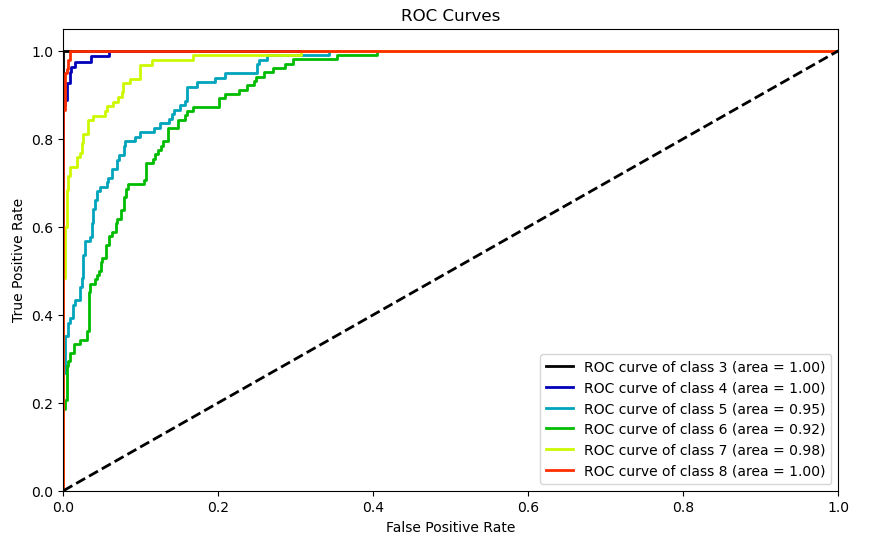
Building Gradient Boosting Classifier (GBC)
GB_model = GradientBoostingClassifier().fit(Train_X_std, Train_Y)
param_dist = {
“n_estimators”:[5,20,100,500],
“max_depth”:[1,3,5,7,9],
“learning_rate”:[0.01,0.1,1,10,100]
}
cv = RepeatedStratifiedKFold(n_splits=10, n_repeats=3, random_state=1)
RCV = RandomizedSearchCV(GB_model, param_dist, n_iter=50, scoring=’f1_weighted’, n_jobs=-1, cv=5, random_state=1)
GB = RCV.fit(Train_X_std, Train_Y).best_estimator_
pred = GB.predict(Test_X_std)
pred_prob = GB.predict_proba(Test_X_std)
Classification_Summary(pred,pred_prob,6)
<<<----------------------------------- Evaluating Gradient Boosting (GB) ----------------------------------->>>

Accuracy = 84.5%
F1 Score = 84.39999999999999%

 Confusion Matrix:
 [[89  0  0  0  0  0]
 [ 0 76  5  0  0  0]
 [ 1  2 68 22  3  1]
 [ 0  2 21 67 10  2]
 [ 0  0  0 14 77  4]
 [ 0  0  0  0  0 97]]

Classification Report:
               precision    recall  f1-score   support

           3       0.99      1.00      0.99        89
           4       0.95      0.94      0.94        81
           5       0.72      0.70      0.71        97
           6       0.65      0.66      0.65       102
           7       0.86      0.81      0.83        95
           8       0.93      1.00      0.97        97

    accuracy                           0.84       561
   macro avg       0.85      0.85      0.85       561
weighted avg       0.84      0.84      0.84       561
Plotting Confusion-Matrix of all the predictive Models
def plot_cm(y_true, y_pred):
cm = confusion_matrix(y_true, y_pred, labels=np.unique(y_true))
cm_sum = np.sum(cm, axis=1, keepdims=True)
cm_perc = cm / cm_sum.astype(float) * 100
annot = np.empty_like(cm).astype(str)
nrows, ncols = cm.shape
for i in range(nrows):
for j in range(ncols):
c = cm[i, j]
p = cm_perc[i, j]
if i == j:
s = cm_sum[i]
annot[i, j] = ‘%.1f%%\n%d/%d’ % (p, c, s)
elif c == 0:
annot[i, j] = ”
else:
annot[i, j] = ‘%.1f%%\n%d’ % (p, c)
cm = pd.DataFrame(cm, index=np.unique(y_true), columns=np.unique(y_true))
cm.columns=labels
cm.index=labels
cm.index.name = ‘Actual’
cm.columns.name = ‘Predicted’
sns.heatmap(cm, annot=annot, fmt=”)# cmap= “GnBu”
def conf_mat_plot(all_models):
plt.figure(figsize=[20,3.5math.ceil(len(all_models)len(labels)/14)])
for i in range(len(all_models)):
    if len(labels)<=4:
        plt.subplot(2,4,i+1)
    else:
        plt.subplot(math.ceil(len(all_models)/3),3,i+1)
    pred = all_models[i].predict(Test_X_std)
    sns.heatmap(confusion_matrix(Test_Y, pred), annot=True, cmap='BuGn', fmt='.0f') #vmin=0,vmax=5
    plt.title(Evaluation_Results.index[i])
plt.tight_layout()
plt.show()
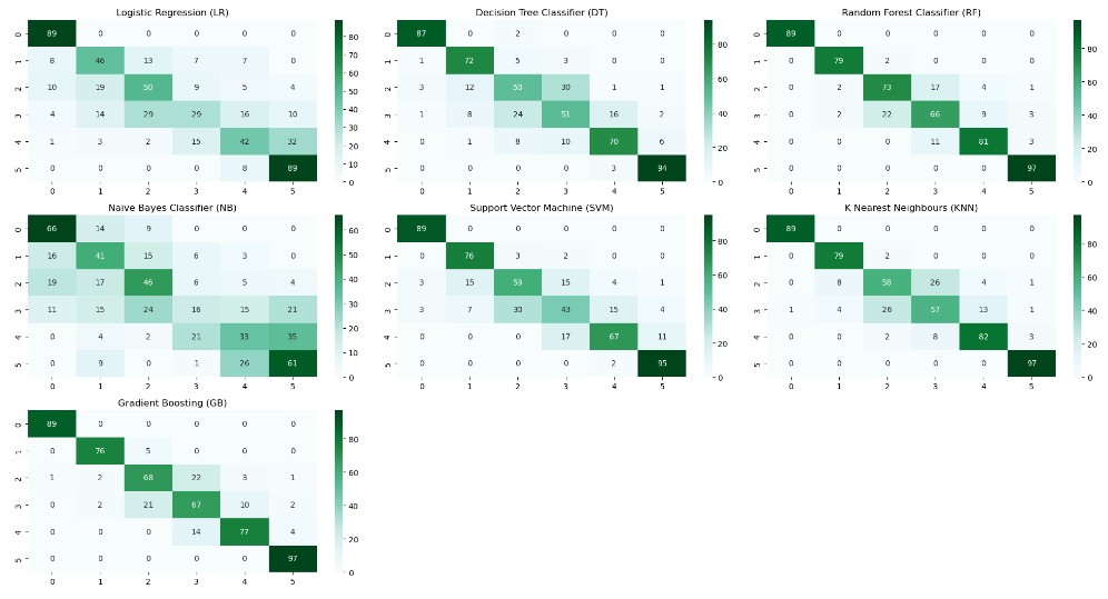
conf_mat_plot([LR,DT,RF,NB,SVM,KNN,GB])
Comparing all the models Scores
print(‘\033[1mML Algorithms Comparison’.center(100))
plt.figure(figsize=[12,8])
sns.heatmap(Evaluation_Results, annot=True, vmin=60, vmax=95, cmap=’Blues’, fmt=’.1f’)
plt.savefig(“mlscoresummary.png”)
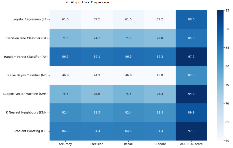
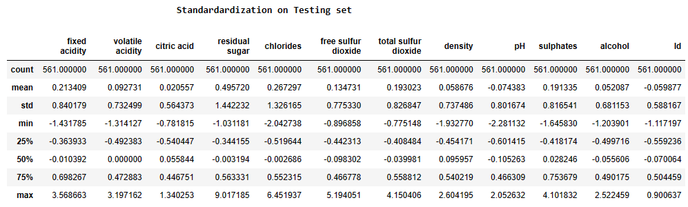
RFC is the best performer for all classes.
Summary
- We compared 7 multi-label ML classifiers to predict wine quality after evaluating their performance based on the accuracy, precision, recall, F1 scores, the ROC-AUC score.
- According to the results, RFC predicted wine quality with higher accuracy.
- Overall, performance of all classifiers improved when model trained and tested using PCA-driven essential variables.
- The usefulness of SMOTE data balancing and importance of feature selection is the key feature in this study.
- We are developing a ML-based API that wine researchers and wine growers can use to predict wine quality based on the important available chemical and physio-chemical compounds in their wines.
Explore More
Semantic Analysis and NLP Visualizations of Wine Reviews
Wine Quality Prediction Using Machine Learning
Embed Socials
Infographic


USA Wine

French Wine
Italian Wine
Spanish Wine

Portuguese Wine


Make a one-time donation
Make a monthly donation
Make a yearly donation
Choose an amount
Or enter a custom amount
Your contribution is appreciated.
Your contribution is appreciated.
Your contribution is appreciated.

Leave a comment