
After over two years of living with Covid-19, we are learning to adapt to a world with this disease.
2022 ends with looming risk of a new coronavirus variant, health experts warn.
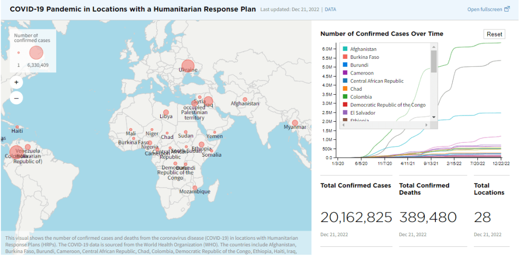
In this post, we explore the statistics on the coronavirus pandemic for every country in the world. The goal is to compare the latest number of confirmed deaths and recovered people of COVID-19 cases Country/Region – Province/State wise. In addition, we invoke COVID-19 Vaccine Sentiment Analysis using Twitter Data for the data science research.
Table of Contents:
- EDA
- Bokeh Plots
- Plotly Impact Analysis
- Vaccine Sentiment Analysis
- Conclusions
- Explore More
- Embed Socials
- Infographic
Let’s set the working directory YOURPATH
import os
os.chdir(‘YOURPATH’)
os. getcwd()
EDA
Referring to the Squarespace Exploratory Data Analysis (EDA), let’s look at the latest number of confirmed deaths and recovered people of Novel Coronavirus cases Country wise.
Let’s import the key libraries and the input dataset
import pandas as pd
covid_data= pd.read_csv(‘https://raw.githubusercontent.com/CSSEGISandData/COVID-19/master/csse_covid_19_data/csse_covid_19_daily_reports/03-17-2020.csv’)
print(covid_data)
print(“\nDataset information:”)
print(covid_data.info())
print(“\nMissing data information:”)
print(covid_data.isna().sum())
 Province/State  Country/Region          Last Update  Confirmed  Deaths  \
0               Hubei           China  2020-03-17T11:53:10      67799    3111
1                 NaN           Italy  2020-03-17T18:33:02      31506    2503
2                 NaN            Iran  2020-03-17T15:13:09      16169     988
3                 NaN           Spain  2020-03-17T20:53:02      11748     533
4                 NaN         Germany  2020-03-17T18:53:02       9257      24
..                ...             ...                  ...        ...     ...
307             Wales  United Kingdom  2020-03-17T11:53:10          0       5
308               NaN           Nauru  2020-03-17T11:53:10          0       0
309              Niue     New Zealand  2020-03-17T11:53:10          0       0
310               NaN          Tuvalu  2020-03-17T11:53:10          0       0
311  Pitcairn Islands  United Kingdom  2020-03-17T11:53:10          0       0

     Recovered  Latitude  Longitude
0        56003   30.9756   112.2707
1         2941   41.8719    12.5674
2         5389   32.4279    53.6880
3         1028   40.4637    -3.7492
4           67   51.1657    10.4515
..         ...       ...        ...
307          0   52.1307    -3.7837
308          0   -0.5228   166.9315
309          0  -19.0544  -169.8672
310          0   -7.1095   177.6493
311          0  -24.3768  -128.3242

[312 rows x 8 columns]

Dataset information:
<class 'pandas.core.frame.DataFrame'>
RangeIndex: 312 entries, 0 to 311
Data columns (total 8 columns):
 #   Column          Non-Null Count  Dtype
---  ------          --------------  -----
 0   Province/State  154 non-null    object
 1   Country/Region  312 non-null    object
 2   Last Update     312 non-null    object
 3   Confirmed       312 non-null    int64
 4   Deaths          312 non-null    int64
 5   Recovered       312 non-null    int64
 6   Latitude        309 non-null    float64
 7   Longitude       309 non-null    float64
dtypes: float64(2), int64(3), object(3)
memory usage: 19.6+ KB
None

Missing data information:
Province/State    158
Country/Region      0
Last Update         0
Confirmed           0
Deaths              0
Recovered           0
Latitude            3
Longitude           3
dtype: int64
Let’s create the Active column
covid_data[‘Active’] = covid_data[‘Confirmed’] – covid_data[‘Deaths’] – covid_data[‘Recovered’]
result = covid_data.groupby(‘Country/Region’)[‘Confirmed’, ‘Deaths’, ‘Recovered’, ‘Active’].sum().reset_index()
print(result)
  Country/Region  Confirmed  Deaths  Recovered  Active
0                       Afghanistan         26       0          1      25
1                           Albania         55       1          0      54
2                           Algeria         60       4         12      44
3                           Andorra         39       0          1      38
4                        Antarctica          0       0          0       0
..                              ...        ...     ...        ...     ...
163                      Uzbekistan         10       0          0      10
164                       Venezuela         33       0          0      33
165                         Vietnam         66       0         16      50
166            Winter Olympics 2022          0       0          0       0
167  occupied Palestinian territory          0       0          0       0

[168 rows x 5 columns]
Let’s plot Deaths vs Confirmed cases
resultdeaths = result.sort_values(‘Deaths’, ascending=False)
resultdeaths10=resultdeaths
import pandas as pd
import plotly.express as px
state_fig = px.scatter(resultdeaths10, x=’Confirmed’, y=’Deaths’, title=’Top COVID-19 Deaths vs Confirmed’, text=’Deaths’,trendline=”ols”)
state_fig.show()

Let’s plot Active vs Recovered
resultdeaths = result.sort_values(‘Active’, ascending=False)
resultdeaths10=resultdeaths
import pandas as pd
import plotly.express as px
state_fig = px.scatter(resultdeaths10, x=’Recovered’, y=’Active’, title=’Top COVID-19 Active vs Recovered’, text=’Active’)
state_fig.show()

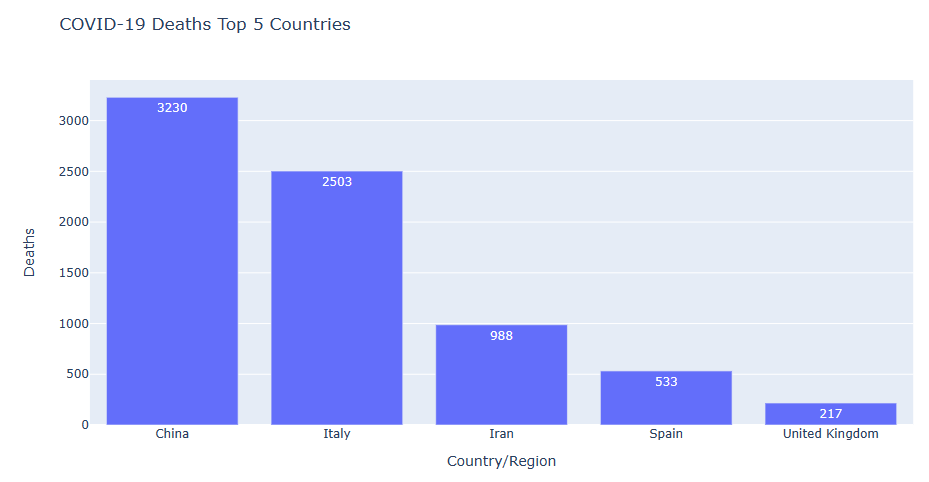
Let’s plot Deaths vs Country/Region
resultdeaths = covid_data.groupby(‘Country/Region’)[‘Deaths’].sum().reset_index().sort_values(‘Deaths’, ascending=False)
resultdeaths10=resultdeaths.head()
import pandas as pd
import plotly.express as px
state_fig = px.bar(resultdeaths10, x=’Country/Region’, y=’Deaths’, title=’COVID-19 Deaths Top 5 Countries’, text=’Deaths’)
state_fig.show()
Let’s group our data
data = covid_data.groupby([‘Country/Region’, ‘Province/State’])[‘Confirmed’, ‘Deaths’, ‘Recovered’].max()
pd.set_option(‘display.max_rows’, None)
print(data)
Confirmed Deaths Recovered
Country/Region Province/State
Australia Australian Capital Territory 2 0 0
From Diamond Princess 0 0 0
New South Wales 210 4 4
Northern Territory 1 0 0
Queensland 78 0 8
South Australia 29 0 3
Tasmania 7 0 0
Victoria 94 0 8
Western Australia 31 1 0
Canada Alberta 74 0 0
British Columbia 103 4 4
Grand Princess 8 0 0
Manitoba 8 0 0
New Brunswick 8 0 0
Newfoundland and Labrador 3 0 0
Nova Scotia 7 0 0
Ontario 507 1 5
Prince Edward Island 1 0 0
Quebec 128 1 0
Saskatchewan 7 0 0
China Anhui 990 6 984
Beijing 456 8 369
Chongqing 576 6 570
Fujian 296 1 295
Gansu 133 2 91
Guangdong 1364 8 1307
Guangxi 253 2 248
Guizhou 147 2 144
Hainan 168 6 161
Hebei 318 6 310
Heilongjiang 482 13 456
Henan 1273 22 1250
Hong Kong 162 4 88
Hubei 67799 3111 56003
Hunan 1018 4 1014
Inner Mongolia 75 1 73
Jiangsu 631 0 631
Jiangxi 935 1 934
Jilin 93 1 92
Liaoning 125 1 120
Macau 12 0 10
Ningxia 75 0 75
Qinghai 18 0 18
Shaanxi 246 3 236
Shandong 761 7 746
Shanghai 358 3 325
Shanxi 133 0 133
Sichuan 540 3 520
Tianjin 136 3 133
Tibet 1 0 1
Unknown 0 0 0
Xinjiang 76 3 73
Yunnan 176 2 172
Zhejiang 1232 1 1216
Cruise Ship Diamond Princess 696 7 325
Denmark Denmark 977 4 1
Faroe Islands 47 0 0
France France 7652 148 12
French Guiana 7 0 0
French Polynesia 3 0 0
Guadeloupe 6 0 0
Mayotte 1 0 0
Reunion 9 0 0
Saint Barthelemy 3 0 0
St Martin 2 0 0
Malaysia Johor 0 0 0
Kedah 0 0 0
Kelantan 0 0 0
Melaka 0 0 0
Negeri Sembilan 0 0 0
Pahang 0 0 0
Perak 0 0 0
Perlis 0 0 0
Pulau Pinang 0 0 0
Sabah 0 0 0
Sarawak 0 0 0
Selangor 0 0 0
Terengganu 0 0 0
Unknown 0 0 0
W.P. Kuala Lumpur 0 0 0
W.P. Labuan 0 0 0
W.P. Putrajaya 0 0 0
Netherlands Curacao 3 0 0
Netherlands 1705 43 2
New Zealand Cook Islands 0 0 0
Niue 0 0 0
US Alabama 39 0 0
Alaska 3 0 0
Arizona 20 0 1
Arkansas 22 0 0
California 698 12 6
Colorado 160 2 0
Connecticut 68 0 0
Delaware 16 0 0
Diamond Princess 47 0 0
District of Columbia 22 0 0
Florida 216 6 0
Georgia 146 1 0
Grand Princess 21 0 0
Guam 3 0 0
Hawaii 10 0 0
Idaho 8 0 0
Illinois 161 1 2
Indiana 30 2 0
Iowa 23 0 0
Kansas 18 1 0
Kentucky 26 1 1
Louisiana 196 4 0
Maine 32 0 0
Maryland 60 0 3
Massachusetts 218 0 1
Michigan 65 0 0
Minnesota 60 0 0
Mississippi 21 0 0
Missouri 11 0 0
Montana 9 0 0
Nebraska 21 0 0
Nevada 56 1 0
New Hampshire 26 0 0
New Jersey 267 3 1
New Mexico 23 0 0
New York 1706 13 0
North Carolina 64 0 0
North Dakota 3 0 0
Ohio 67 0 0
Oklahoma 19 0 0
Oregon 66 1 0
Pennsylvania 112 0 0
Puerto Rico 5 0 0
Rhode Island 23 0 0
South Carolina 47 1 0
South Dakota 11 1 0
Tennessee 74 0 0
Texas 110 1 0
Utah 51 0 0
Vermont 12 0 0
Virgin Islands 2 0 0
Virginia 67 2 0
Washington 1076 55 1
West Virginia 1 0 0
Wisconsin 72 0 1
Wyoming 11 0 0
Ukraine Unknown 0 0 0
United Kingdom Cayman Islands 1 1 0
Channel Islands 0 0 0
England 0 198 0
Gibraltar 3 0 1
Guernsey 0 0 0
Jersey 0 0 0
Northern Ireland 0 0 0
Pitcairn Islands 0 0 0
Scotland 0 11 0
Unknown 1950 2 52
Wales 0 5 0
Let’s select China
c_data = covid_data[covid_data[‘Country/Region’]==’China’]
c_data = c_data[[‘Province/State’, ‘Confirmed’, ‘Deaths’, ‘Recovered’]]
result = c_data.sort_values(by=’Confirmed’, ascending=False)
result = result.reset_index(drop=True)
print(result)
 Province/State  Confirmed  Deaths  Recovered
0            Hubei      67799    3111      56003
1        Guangdong       1364       8       1307
2            Henan       1273      22       1250
3         Zhejiang       1232       1       1216
4            Hunan       1018       4       1014
5            Anhui        990       6        984
6          Jiangxi        935       1        934
7         Shandong        761       7        746
8          Jiangsu        631       0        631
9        Chongqing        576       6        570
10         Sichuan        540       3        520
11    Heilongjiang        482      13        456
12         Beijing        456       8        369
13        Shanghai        358       3        325
14           Hebei        318       6        310
15          Fujian        296       1        295
16         Guangxi        253       2        248
17         Shaanxi        246       3        236
18          Yunnan        176       2        172
19          Hainan        168       6        161
20       Hong Kong        162       4         88
21         Guizhou        147       2        144
22         Tianjin        136       3        133
23           Gansu        133       2         91
24          Shanxi        133       0        133
25        Liaoning        125       1        120
26           Jilin         93       1         92
27        Xinjiang         76       3         73
28  Inner Mongolia         75       1         73
29         Ningxia         75       0         75
30         Qinghai         18       0         18
31           Macau         12       0         10
32           Tibet          1       0          1
33         Unknown          0       0          0
Let’s plot Confirmed per Province
resultdeaths10=result
import pandas as pd
import plotly.express as px
state_fig = px.bar(resultdeaths10, x=’Province/State’, y=’Confirmed’, title=’COVID-19 Confirmed Top 10 Provinces’)
state_fig.show()

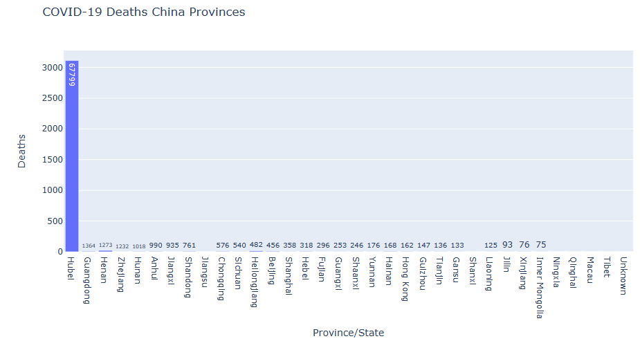
Let’s plot Deaths per Province
resultdeaths10=result
import pandas as pd
import plotly.express as px
state_fig = px.bar(resultdeaths10, x=’Province/State’, y=’Deaths’, title=’COVID-19 Deaths China Provinces’)
state_fig.show()
Let’s plot Recovered per Province
resultdeaths10=result
import pandas as pd
import plotly.express as px
state_fig = px.bar(resultdeaths10, x=’Province/State’, y=’Recovered’, title=’COVID-19 Recovered China Provinces’)
state_fig.show()

Let’s select subset Deaths>0 vs Country/Region
data = covid_data.groupby(‘Country/Region’)[‘Confirmed’, ‘Deaths’, ‘Recovered’].sum().reset_index()
result = data[data[‘Deaths’]>0][[‘Country/Region’, ‘Deaths’]]
print(result)
Country/Region  Deaths
1               Albania       1
2               Algeria       4
6             Argentina       2
9             Australia       5
10              Austria       3
11           Azerbaijan       1
12              Bahrain       1
16              Belgium      10
21               Brazil       1
23             Bulgaria       2
27               Canada       6
30                China    3230
37          Cruise Ship       7
41              Denmark       4
42   Dominican Republic       1
43              Ecuador       2
44                Egypt       4
49              Finland       4
50               France     148
54              Germany      24
56               Greece       5
60            Guatemala       1
63               Guyana       1
66              Hungary       1
67              Iceland       1
68                India       3
69            Indonesia       5
70                 Iran     988
71                 Iraq      11
72              Ireland       2
74                Italy    2503
76                Japan      29
83         Korea, South      81
87              Lebanon       3
91           Luxembourg       1
95           Martinique       1
103             Morocco       2
107         Netherlands      43
111              Norway       3
115              Panama       1
117                Peru       9
118         Philippines      12
119              Poland       5
120            Portugal       1
130          San Marino       9
137            Slovenia       1
140               Spain     533
142               Sudan       1
145              Sweden       7
146         Switzerland      40
147             Taiwan*       1
149            Thailand       1
156              Turkey       1
158                  US     108
159             Ukraine       2
161      United Kingdom     217
Let’s select subset Recovered=0 vs Country/Region
data = covid_data.groupby(‘Country/Region’)[‘Confirmed’, ‘Deaths’, ‘Recovered’].sum().reset_index()
result = data[data[‘Recovered’]==0][[‘Country/Region’, ‘Confirmed’, ‘Deaths’, ‘Recovered’]]
print(result)
Country/Region  Confirmed  Deaths  Recovered
1                             Albania         55       1          0
4                          Antarctica          0       0          0
5                 Antigua and Barbuda          1       0          0
8                               Aruba          3       0          0
14                           Barbados          2       0          0
17                              Benin          1       0          0
18                             Bhutan          1       0          0
19                            Bolivia         11       0          0
22                             Brunei         56       0          0
23                           Bulgaria         67       2          0
24                       Burkina Faso         15       0          0
26                           Cameroon         10       0          0
28           Central African Republic          1       0          0
29                              Chile        201       0          0
32                Congo (Brazzaville)          1       0          0
33                   Congo (Kinshasa)          3       0          0
34                         Costa Rica         41       0          0
38                               Cuba          5       0          0
39                             Cyprus         40       0          0
42                 Dominican Republic         21       1          0
43                            Ecuador         58       2          0
45                  Equatorial Guinea          1       0          0
47                           Eswatini          1       0          0
48                           Ethiopia          5       0          0
51                      French Guiana         11       0          0
52                              Gabon          1       0          0
55                              Ghana          7       0          0
57                          Greenland          1       0          0
58                         Guadeloupe         18       0          0
59                               Guam          3       0          0
60                          Guatemala          6       1          0
61                           Guernsey          0       0          0
62                             Guinea          1       0          0
63                             Guyana          7       1          0
64                           Holy See          1       0          0
65                           Honduras          8       0          0
67                            Iceland        220       1          0
77                             Jersey          0       0          0
79                         Kazakhstan         33       0          0
80                              Kenya          3       0          0
81                           Kiribati          0       0          0
82                       Korea, North          0       0          0
84                             Kosovo          2       0          0
88                            Liberia          5       0          0
89                      Liechtenstein         19       0          0
91                         Luxembourg        140       1          0
92                           Malaysia          0       0          0
93                           Maldives         13       0          0
95                         Martinique         16       1          0
96                         Mauritania          1       0          0
97                            Mayotte          1       0          0
100                            Monaco          7       0          0
101                          Mongolia          4       0          0
102                        Montenegro          2       0          0
104                           Namibia          2       0          0
105                             Nauru          0       0          0
108                       New Zealand         12       0          0
109                           Nigeria          3       0          0
114                             Palau          0       0          0
115                            Panama         69       1          0
116                          Paraguay         11       0          0
121                       Puerto Rico          0       0          0
123             Republic of the Congo          0       0          0
124                           Reunion          9       0          0
127                            Rwanda          7       0          0
128                       Saint Lucia          2       0          0
129  Saint Vincent and the Grenadines          1       0          0
134                        Seychelles          8       0          0
136                          Slovakia         72       0          0
137                          Slovenia        275       1          0
138                           Somalia          1       0          0
139                      South Africa         62       0          0
142                             Sudan          1       1          0
143              Summer Olympics 2020          0       0          0
144                          Suriname          1       0          0
148                          Tanzania          1       0          0
150                       The Bahamas          1       0          0
151                        The Gambia          1       0          0
152                              Togo          1       0          0
153                             Tonga          0       0          0
154               Trinidad and Tobago          5       0          0
155                           Tunisia         24       0          0
156                            Turkey         47       1          0
157                            Tuvalu          0       0          0
159                           Ukraine         14       2          0
162                           Uruguay         29       0          0
163                        Uzbekistan         10       0          0
164                         Venezuela         33       0          0
166              Winter Olympics 2022          0       0          0
167    occupied Palestinian territory          0       0          0
Let’s check the condition data[data[‘Confirmed’]==data[‘Deaths’]]
data = covid_data.groupby(‘Country/Region’)[‘Confirmed’, ‘Deaths’, ‘Recovered’].sum().reset_index()
result = data[data[‘Confirmed’]==data[‘Deaths’]]
result = result[[‘Country/Region’, ‘Confirmed’, ‘Deaths’]]
result = result.sort_values(‘Confirmed’, ascending=False)
result = result[result[‘Confirmed’]>0]
result = result.reset_index(drop=True)
print(result)
Country/Region  Confirmed  Deaths
0          Sudan          1       1
Let’s check the condition data[data[‘Confirmed’]==data[‘Recovered’]]
data = covid_data.groupby(‘Country/Region’)[‘Confirmed’, ‘Deaths’, ‘Recovered’].sum().reset_index()
result = data[data[‘Confirmed’]==data[‘Recovered’]]
result = result[[‘Country/Region’, ‘Confirmed’, ‘Recovered’]]
result = result.sort_values(‘Confirmed’, ascending=False)
result = result[result[‘Confirmed’]>0]
result = result.reset_index(drop=True)
print(result)
 Country/Region  Confirmed  Recovered
0          Nepal          1          1
Let’s select top 10 Confirmed countries
result = covid_data.groupby(‘Country/Region’).max().sort_values(by=’Confirmed’, ascending=False)[:10]
pd.set_option(‘display.max_column’, None)
print(result)
      Last Update  Confirmed  Deaths  Recovered  Latitude  \
Country/Region
China           2020-03-17T12:13:13      67799    3111      56003   47.8620
Italy           2020-03-17T18:33:02      31506    2503       2941   41.8719
Iran            2020-03-17T15:13:09      16169     988       5389   32.4279
Spain           2020-03-17T20:53:02      11748     533       1028   40.4637
Germany         2020-03-17T18:53:02       9257      24         67   51.1657
Korea, South    2020-03-17T10:33:03       8320      81       1407   35.9078
France          2020-03-17T19:13:08       7652     148         12   46.2276
Switzerland     2020-03-17T16:33:04       2700      40          4   46.8182
United Kingdom  2020-03-17T15:13:09       1950     198         52   56.4907
US              2020-03-17T23:53:03       1706      55          6   61.3707

                Longitude  Active
Country/Region
China            127.7615    8685
Italy             12.5674   26062
Iran              53.6880    9792
Spain             -3.7492   10187
Germany           10.4515    9166
Korea, South     127.7669    6832
France            55.2471    7492
Switzerland        8.2275    2656
United Kingdom    -1.1743    1896
US               144.7937    1693
Let’s plot Total Deaths(>150), Confirmed, Recovered and Active Cases by Country (top 10 countries)
import pandas as pd
import matplotlib.pyplot as plt
covid_data= pd.read_csv(‘https://raw.githubusercontent.com/CSSEGISandData/COVID-19/master/csse_covid_19_data/csse_covid_19_daily_reports/03-19-2020.csv’, usecols = [‘Last Update’, ‘Country/Region’, ‘Confirmed’, ‘Deaths’, ‘Recovered’])
covid_data[‘Active’] = covid_data[‘Confirmed’] – covid_data[‘Deaths’] – covid_data[‘Recovered’]
r_data = covid_data.groupby([“Country/Region”])[“Deaths”, “Confirmed”, “Recovered”, “Active”].sum().reset_index()
r_data = r_data.sort_values(by=’Deaths’, ascending=False)
r_data = r_data[r_data[‘Deaths’]>50]
plt.figure(figsize=(15, 5))
plt.plot(r_data[‘Country/Region’], r_data[‘Deaths’],color=’red’)
plt.plot(r_data[‘Country/Region’], r_data[‘Confirmed’],color=’green’)
plt.plot(r_data[‘Country/Region’], r_data[‘Recovered’], color=’blue’)
plt.plot(r_data[‘Country/Region’], r_data[‘Active’], color=’black’)
plt.title(‘Total Deaths(>150), Confirmed, Recovered and Active Cases by Country’)
plt.show()

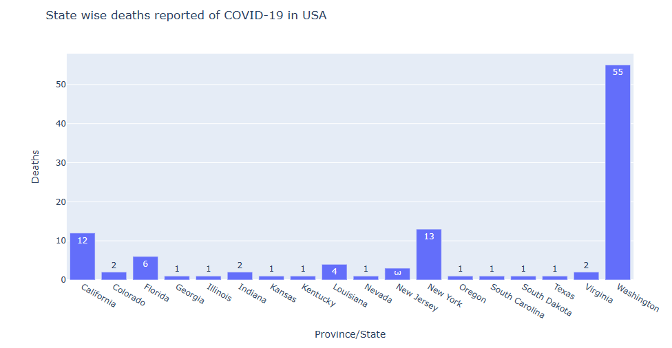
Let’s select US and plot Deaths per State
import pandas as pd
import plotly.express as px
covid_data= pd.read_csv(‘https://raw.githubusercontent.com/CSSEGISandData/COVID-19/master/csse_covid_19_data/csse_covid_19_daily_reports/03-17-2020.csv’)
us_data = covid_data[covid_data[‘Country/Region’]==’US’].drop([‘Country/Region’,’Latitude’, ‘Longitude’], axis=1)
us_data = us_data[us_data.sum(axis = 1) > 0]
us_data = us_data.groupby([‘Province/State’])[‘Deaths’].sum().reset_index()
us_data_death = us_data[us_data[‘Deaths’] > 0]
state_fig = px.bar(us_data_death, x=’Province/State’, y=’Deaths’, title=’State wise deaths reported of COVID-19 in USA’, text=’Deaths’)
state_fig.show()
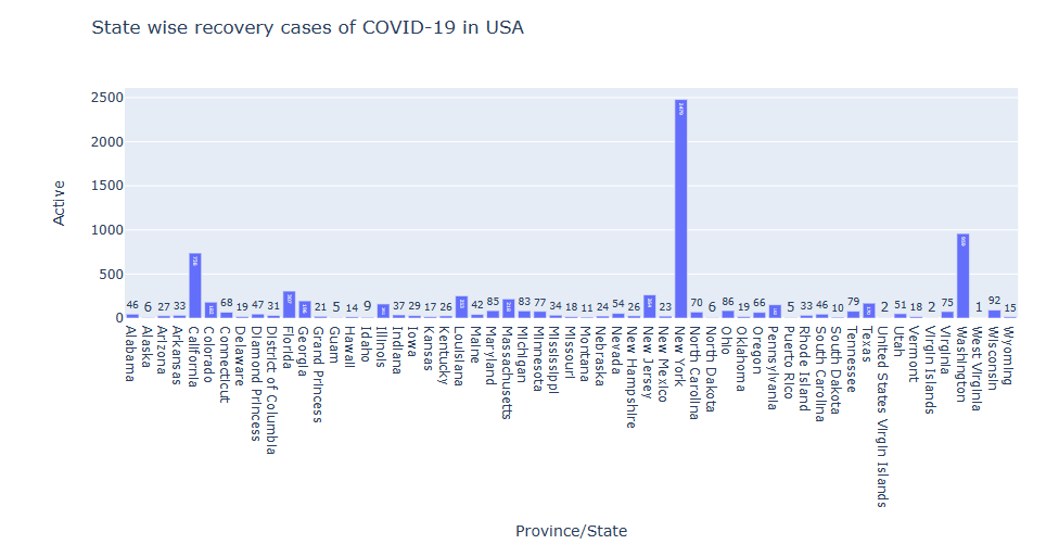
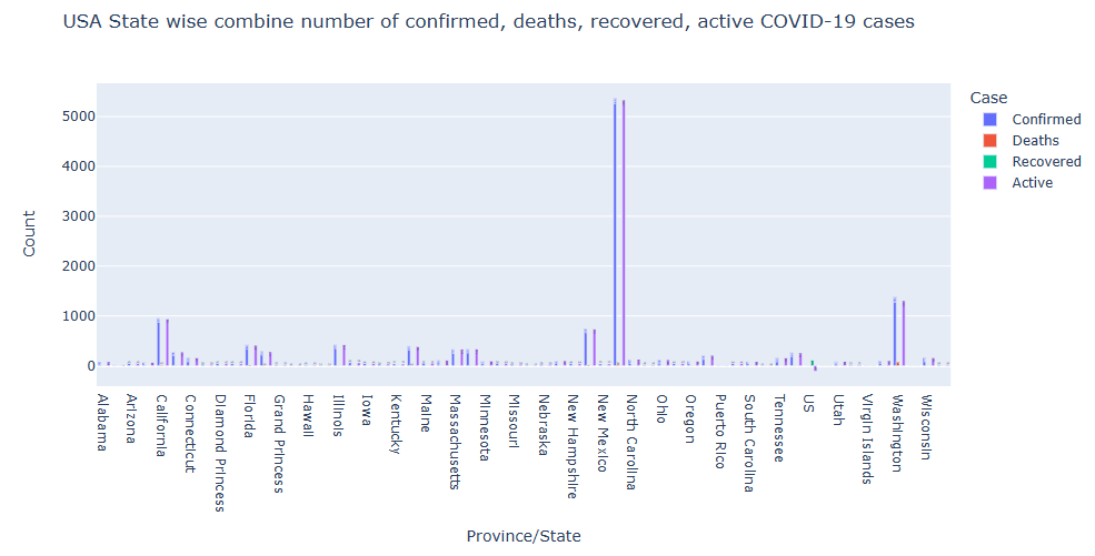
Let’s plot US states Recovery
import pandas as pd
import plotly.express as px
covid_data= pd.read_csv(‘https://raw.githubusercontent.com/CSSEGISandData/COVID-19/master/csse_covid_19_data/csse_covid_19_daily_reports/03-18-2020.csv’)
covid_data[‘Active’] = covid_data[‘Confirmed’] – covid_data[‘Deaths’] – covid_data[‘Recovered’]
us_data = covid_data[covid_data[‘Country/Region’]==’US’].drop([‘Country/Region’,’Latitude’, ‘Longitude’], axis=1)
us_data = us_data[us_data.sum(axis = 1) > 0]
us_data = us_data.groupby([‘Province/State’])[‘Active’].sum().reset_index()
us_data_death = us_data[us_data[‘Active’] > 0]
state_fig = px.bar(us_data_death, x=’Province/State’, y=’Active’, title=’State wise recovery cases of COVID-19 in USA’, text=’Active’)
state_fig.show()
Let’s plot Confirmed, Deaths, Active, and Recovered for US states
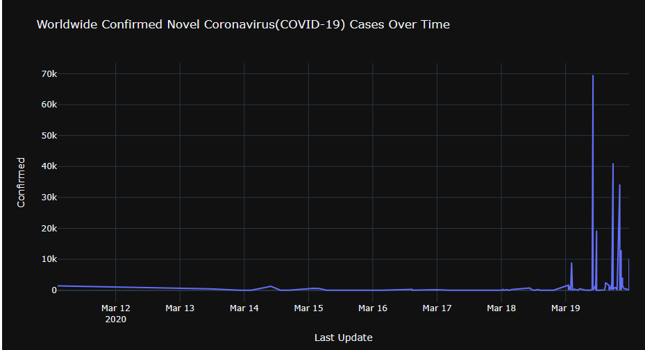
Let’s plot Worldwide Confirmed Novel Coronavirus(COVID-19) Cases Over Time
import pandas as pd
import plotly.express as px
import plotly.io as pio
pio.templates.default = “plotly_dark”
covid_data= pd.read_csv(‘https://raw.githubusercontent.com/CSSEGISandData/COVID-19/master/csse_covid_19_data/csse_covid_19_daily_reports/03-19-2020.csv’)
grouped = covid_data.groupby(‘Last Update’)[‘Last Update’, ‘Confirmed’, ‘Deaths’].sum().reset_index()
fig = px.line(grouped, x=”Last Update”, y=”Confirmed”,
title=”Worldwide Confirmed Novel Coronavirus(COVID-19) Cases Over Time”)
fig.show()
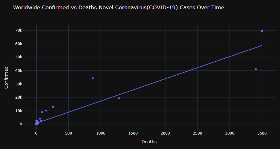
Let’s look at the scatter plot Worldwide Confirmed vs Deaths Novel Coronavirus(COVID-19) Cases Over Time (with the linear trend)
fig = px.scatter(grouped, x=”Deaths”, y=”Confirmed”,
title=”Worldwide Confirmed vs Deaths Novel Coronavirus(COVID-19) Cases Over Time”,trendline=”ols”)
fig.show()
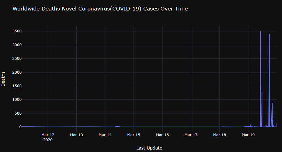
Let’s plot Worldwide Deaths Novel Coronavirus(COVID-19) Cases Over Time
fig = px.line(grouped, x=”Last Update”, y=”Deaths”,
title=”Worldwide Deaths Novel Coronavirus(COVID-19) Cases Over Time”)
fig.show()
Bokeh Plots
Let’s invoke the Bokeh library to see how Asia is doing against COVID-19
We begin with importing the key libraries
import gc
import numpy as np
import pandas as pd
import matplotlib.pyplot as plt
import seaborn as sns
from bokeh.plotting import figure
from bokeh.models import LabelSet, ColumnDataSource
from bokeh.io import show, output_notebook
from bokeh.io import output_notebook
from bokeh.resources import INLINE
from bokeh.layouts import row, column
output_notebook(INLINE)
import warnings
warnings.filterwarnings(‘ignore’)
Loading BokehJS …
Importing the dataset
df = pd.read_csv(‘AsiaCases_.csv’)
df.head().style.background_gradient(cmap=’RdGy’)

Checking for any missing values
df.isnull().sum()
ID                       0
Country                  0
TotalCases               0
TotalDeaths              1
TotalRecovered           0
ActiveCases              0
TotalCasesPerMillion     0
TotalDeathsPerMillion    1
TotalTests               1
TotalTestsPerMillion     1
TotalPopulation          0
dtype: int64
Dropping the countries with missing data
df.dropna(axis=0, inplace=True)
and checking the descriptive statistics
df.describe().T

df.info()
<class 'pandas.core.frame.DataFrame'>
Int64Index: 47 entries, 0 to 48
Data columns (total 11 columns):
 #   Column                 Non-Null Count  Dtype
---  ------                 --------------  -----
 0   ID                     47 non-null     int64
 1   Country                47 non-null     object
 2   TotalCases             47 non-null     int64
 3   TotalDeaths            47 non-null     float64
 4   TotalRecovered         47 non-null     int64
 5   ActiveCases            47 non-null     int64
 6   TotalCasesPerMillion   47 non-null     int64
 7   TotalDeathsPerMillion  47 non-null     float64
 8   TotalTests             47 non-null     float64
 9   TotalTestsPerMillion   47 non-null     float64
 10  TotalPopulation        47 non-null     int64
dtypes: float64(4), int64(6), object(1)
memory usage: 4.4+ KB
Checking the number of rows and columns
print(‘Number of rows:’, df.shape[0])
print(‘Number of columns:’, df.shape[1])
Number of rows: 47
Number of columns: 11
Let’s drop the ID column
df.drop(columns=’ID’, axis=1, inplace=True)
Let’s plot top 10 countries with the highest number of cases
df_high_cases = df[[‘Country’,’TotalCases’,’TotalPopulation’]].sort_values(by=’TotalCases’, ascending=False)
df_high_cases = df_high_cases.iloc[:10,:]
df_high_cases[‘perc’] = round((df_high_cases[‘TotalCases’] / df_high_cases[‘TotalPopulation’]) * 100, 1)
df_high_cases[‘perc’] = df_high_cases[‘perc’].apply(str)
df_high_cases[‘perc’] = df_high_cases[‘perc’]+’%’
Our x and y axis
country = list(df_high_cases[‘Country’].values)
pop = list(df_high_cases[‘TotalPopulation’].values)
case = list(df_high_cases[‘TotalCases’].values)
perc = list(df_high_cases[‘perc’].values)
For the Cases
p1 = figure(x_range=country, y_range=[0,40000000], height=500, width=1000, title=”Top 10 Countries in terms of Covid-19 Cases”)
p1.background_fill_color = “#efefef”
p1.vbar(x=country, top=case, width=0.9, color=’#db0000′,
alpha=[1,0.9,0.8,0.7,0.6,0.5,0.4,0.3,0.2,0.1],
line_color=”black”,line_width=3)
source = ColumnDataSource(data=dict(y=case,
x=country,
names=perc,
text_font_size=[’20px’],
text_alpha=[1,0.9,0.8,0.7,0.6,0.5,0.4,0.3,0.2,0.2]))
labels = LabelSet(x=’x’, y=’y’, text=’names’, source=source, text_font_size=’text_font_size’, text_alpha=’text_alpha’, x_offset=-18)
p1.ygrid.grid_line_color = None
p1.xgrid.grid_line_color = None
p1.title.text_font_size = ’18pt’
p1.add_layout(labels, place=’center’)
p1.xaxis.major_label_text_font_size = “12pt”
Let’s call show(column(p1, p2))
gc.collect()
show(p1)

Let’s plot top 10 countries with highest number of deaths
df_high_death = df[[‘Country’,’TotalDeaths’,’TotalPopulation’]].sort_values(by=’TotalDeaths’, ascending=False)
df_high_death = df_high_death.iloc[:10,:]
df_high_death[‘perc’] = round((df_high_death[‘TotalDeaths’] / df_high_death[‘TotalPopulation’]) * 100, 3)
df_high_death[‘perc’] = df_high_death[‘perc’].apply(str)
df_high_death[‘perc’] = df_high_death[‘perc’]+’%’
Our x and y axis
country = list(df_high_death[‘Country’].values)
pop = list(df_high_cases[‘TotalPopulation’].values)
case = list(df_high_death[‘TotalDeaths’].values)
perc = list(df_high_death[‘perc’].values)
For the Cases
p1 = figure(x_range=country, y_range=[0,500000], height=500, width=1000, title=”Top 10 Countries in terms of Covid-19 Deaths”)
p1.background_fill_color = “#efefef”
p1.vbar(x=country, top=case, width=0.9, color=’#db0000′,
alpha=[1,0.9,0.8,0.7,0.6,0.5,0.4,0.3,0.2,0.1],
line_color=”black”,line_width=3)
source = ColumnDataSource(data=dict(y=case,
x=country,
names=perc,
text_font_size=[’20px’],
text_alpha=[1,0.9,0.8,0.7,0.6,0.5,0.4,0.3,0.2,0.2]))
labels = LabelSet(x=’x’, y=’y’, text=’names’, source=source, text_font_size=’text_font_size’, text_alpha=’text_alpha’, x_offset=-25)
p1.ygrid.grid_line_color = None
p1.xgrid.grid_line_color = None
p1.title.text_font_size = ’18pt’
p1.add_layout(labels, place=’center’)
p1.xaxis.major_label_text_font_size = “12pt”
gc.collect()
show(p1)

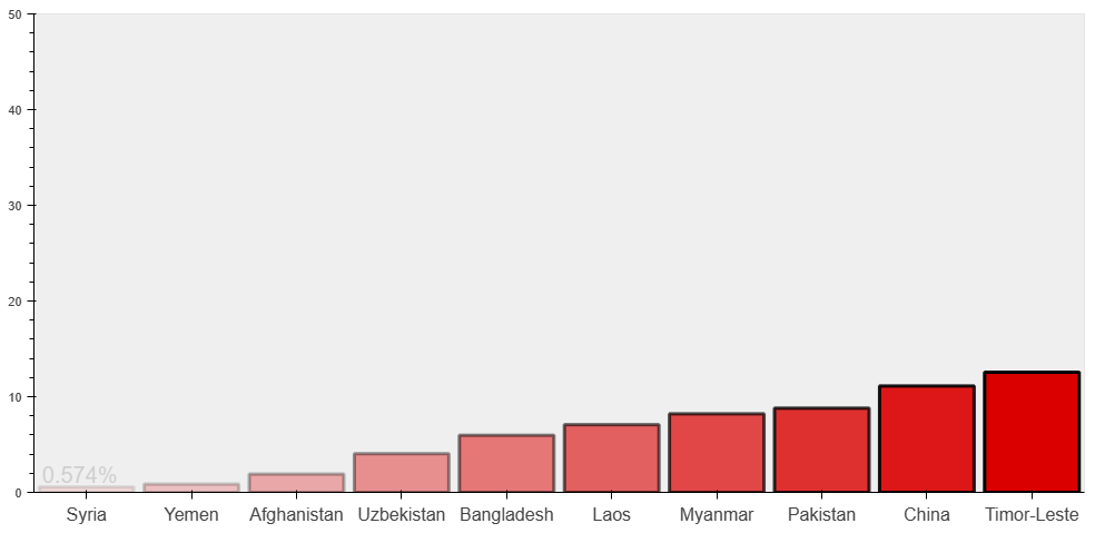
Let’s plot top 10 Asian countries with the lowest number of tests
df_low_test = df[[‘Country’,’TotalTests’,’TotalPopulation’]]
df_low_test[‘perc’] = round((df_low_test[‘TotalTests’] / df_low_test[‘TotalPopulation’]) * 100, 3)
df_low_test = df_low_test.sort_values(by=’perc’, ascending=True).iloc[:10,:]
df_low_test[‘perc_’] = df_low_test[‘perc’].apply(str)
df_low_test[‘perc_’] = df_low_test[‘perc_’]+’%’
Our x and y axis
country = list(df_low_test[‘Country’].values)
pop = list(df_high_cases[‘TotalPopulation’].values)
case = list(df_low_test[‘TotalTests’].values)
perc = list(df_low_test[‘perc’].values)
perc_ = list(df_low_test[‘perc_’].values)
For the Cases
p1 = figure(x_range=country, y_range=[0,50], height=500, width=1000, title=”Bottom 10 Countries in terms of Covid-19 Test/Population”)
p1.background_fill_color = “#efefef”
p1.vbar(x=country, top=perc, width=0.9, color=’#db0000′,
alpha=[0.1,0.2,0.3,0.4,0.5,0.6,0.7,0.8,0.9,1],
line_color=”black”,line_width=3)
source = ColumnDataSource(data=dict(y=perc,
x=country,
names=perc_,
text_font_size=[’20px’],
text_alpha=[0.2,0.2,0.3,0.4,0.5,0.6,0.7,0.8,0.9,1]))
labels = LabelSet(x=’x’, y=’y’, text=’names’, source=source, text_font_size=’text_font_size’, text_alpha=’text_alpha’, x_offset=-40)
p1.ygrid.grid_line_color = None
p1.xgrid.grid_line_color = None
p1.title.text_font_size = ’18pt’
p1.add_layout(labels, place=’center’)
p1.xaxis.major_label_text_font_size = “12pt”
gc.collect()
show(p1)
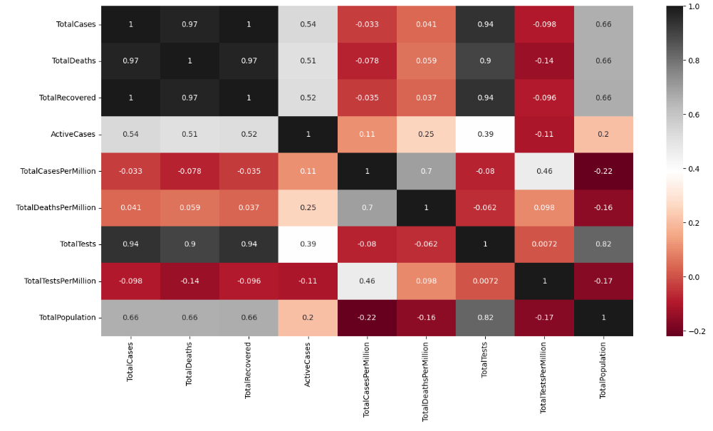
Checking if there are any data correlations
heat = df.corr()
plt.figure(figsize=[16,8])
sns.heatmap(heat, annot=True, cmap=’RdGy’)
gc.collect()
plt.show()
Let’s plot Total Deaths to Recovery ratio
df_ded_reco = df[[‘Country’,’TotalDeaths’,’TotalRecovered’]]
df_ded_reco[‘DeadRecovRatio’] = round(df_ded_reco[‘TotalDeaths’]/df_ded_reco[‘TotalRecovered’], 4)
df_ded_reco = df_ded_reco.sort_values(by=’DeadRecovRatio’, ascending=False).iloc[:10,:]
Our x and y axis
country = list(df_ded_reco[‘Country’].values)
case = list(df_ded_reco[‘DeadRecovRatio’].values)
For the Cases
p1 = figure(x_range=country, y_range=[0,0.5], height=500, width=1000, title=”Top 10 Countries in terms of Death/Recovery Ratio”)
p1.background_fill_color = “#efefef”
p1.vbar(x=country, top=case, width=0.9, color=’#db0000′,
alpha=[1,0.9,0.8,0.7,0.6,0.5,0.4,0.3,0.2,0.2],
line_color=”black”,line_width=3)
p1.ygrid.grid_line_color = None
p1.xgrid.grid_line_color = None
p1.title.text_font_size = ’18pt’
gc.collect()
show(p1)

Plotly Impact Analysis
Let’s implement the COVID-19 impact analysis using Plotly.
Let’s set the working directory YOURPATH, import key libraries and input COVID-19 data
import os
os.chdir(‘C:/Users/adrou/OneDrive/Documents/COVIDAMAN’) # Set working directory
os. getcwd()
import pandas as pd
import plotly.express as px
import plotly.graph_objects as go
data = pd.read_csv(“transformed_data.csv”)
data2 = pd.read_csv(“raw_data.csv”)
print(data)
 CODE      COUNTRY        DATE    HDI        TC        TD       STI  \
0      AFG  Afghanistan  2019-12-31  0.498  0.000000  0.000000  0.000000
1      AFG  Afghanistan  2020-01-01  0.498  0.000000  0.000000  0.000000
2      AFG  Afghanistan  2020-01-02  0.498  0.000000  0.000000  0.000000
3      AFG  Afghanistan  2020-01-03  0.498  0.000000  0.000000  0.000000
4      AFG  Afghanistan  2020-01-04  0.498  0.000000  0.000000  0.000000
...    ...          ...         ...    ...       ...       ...       ...
50413  ZWE     Zimbabwe  2020-10-15  0.535  8.994048  5.442418  4.341855
50414  ZWE     Zimbabwe  2020-10-16  0.535  8.996528  5.442418  4.341855
50415  ZWE     Zimbabwe  2020-10-17  0.535  8.999496  5.442418  4.341855
50416  ZWE     Zimbabwe  2020-10-18  0.535  9.000853  5.442418  4.341855
50417  ZWE     Zimbabwe  2020-10-19  0.535  9.005405  5.442418  4.341855

             POP    GDPCAP
0      17.477233  7.497754
1      17.477233  7.497754
2      17.477233  7.497754
3      17.477233  7.497754
4      17.477233  7.497754
...          ...       ...
50413  16.514381  7.549491
50414  16.514381  7.549491
50415  16.514381  7.549491
50416  16.514381  7.549491
50417  16.514381  7.549491

[50418 rows x 9 columns]
Let’s check value_counts() per country
data[“COUNTRY”].value_counts()
Afghanistan        294
Indonesia          294
Macedonia          294
Luxembourg         294
Lithuania          294
                  ...
Tajikistan         172
Comoros            171
Lesotho            158
Hong Kong           51
Solomon Islands      4
Name: COUNTRY, Length: 210, dtype: int64
The total number of countries is
data[“COUNTRY”].value_counts().mode()
0    294
Name: COUNTRY, dtype: int64
Aggregating the data
code = data[“CODE”].unique().tolist()
country = data[“COUNTRY”].unique().tolist()
hdi = []
tc = []
td = []
sti = []
population = data[“POP”].unique().tolist()
gdp = []
for i in country:
hdi.append((data.loc[data[“COUNTRY”] == i, “HDI”]).sum()/294)
tc.append((data2.loc[data2[“location”] == i, “total_cases”]).sum())
td.append((data2.loc[data2[“location”] == i, “total_deaths”]).sum())
sti.append((data.loc[data[“COUNTRY”] == i, “STI”]).sum()/294)
population.append((data2.loc[data2[“location”] == i, “population”]).sum()/294)
aggregated_data = pd.DataFrame(list(zip(code, country, hdi, tc, td, sti, population)),
columns = [“Country Code”, “Country”, “HDI”,
“Total Cases”, “Total Deaths”,
“Stringency Index”, “Population”])
print(aggregated_data.head())
 Country Code      Country       HDI  Total Cases  Total Deaths  \
0          AFG  Afghanistan  0.498000    5126433.0      165875.0
1          ALB      Albania  0.600765    1071951.0       31056.0
2          DZA      Algeria  0.754000    4893999.0      206429.0
3          AND      Andorra  0.659551     223576.0        9850.0
4          AGO       Angola  0.418952     304005.0       11820.0

   Stringency Index  Population
0          3.049673   17.477233
1          3.005624   14.872537
2          3.195168   17.596309
3          2.677654   11.254996
4          2.965560   17.307957
Sorting Data According to Total Cases
data = aggregated_data.sort_values(by=[“Total Cases”], ascending=False)
print(data.head())
Country Code        Country      HDI  Total Cases  Total Deaths  \
200          USA  United States  0.92400  746014098.0    26477574.0
27           BRA         Brazil  0.75900  425704517.0    14340567.0
90           IND          India  0.64000  407771615.0     7247327.0
157          RUS         Russia  0.81600  132888951.0     2131571.0
150          PER           Peru  0.59949   74882695.0     3020038.0

     Stringency Index  Population
200          3.350949   19.617637
27           3.136028   19.174732
90           3.610552   21.045353
157          3.380088   18.798668
150          3.430126   17.311165
Let’s select top 10 Countries with Highest Covid Cases
data = data.head(10)
print(data)
 Country Code         Country       HDI  Total Cases  Total Deaths  \
200          USA   United States  0.924000  746014098.0    26477574.0
27           BRA          Brazil  0.759000  425704517.0    14340567.0
90           IND           India  0.640000  407771615.0     7247327.0
157          RUS          Russia  0.816000  132888951.0     2131571.0
150          PER            Peru  0.599490   74882695.0     3020038.0
125          MEX          Mexico  0.774000   74347548.0     7295850.0
178          ESP           Spain  0.887969   73717676.0     5510624.0
175          ZAF    South Africa  0.608653   63027659.0     1357682.0
42           COL        Colombia  0.581847   60543682.0     1936134.0
199          GBR  United Kingdom  0.922000   59475032.0     7249573.0

     Stringency Index  Population
200          3.350949   19.617637
27           3.136028   19.174732
90           3.610552   21.045353
157          3.380088   18.798668
150          3.430126   17.311165
125          3.019289   18.674802
178          3.393922   17.660427
175          3.364333   17.898266
42           3.357923   17.745037
199          3.353883   18.033340
Let’s compare country GDP before/during COVID
data[“GDP Before Covid”] = [65279.53, 8897.49, 2100.75,
11497.65, 7027.61, 9946.03,
29564.74, 6001.40, 6424.98, 42354.41]
data[“GDP During Covid”] = [63543.58, 6796.84, 1900.71,
10126.72, 6126.87, 8346.70,
27057.16, 5090.72, 5332.77, 40284.64]
print(data)
Country Code         Country       HDI  Total Cases  Total Deaths  \
200          USA   United States  0.924000  746014098.0    26477574.0
27           BRA          Brazil  0.759000  425704517.0    14340567.0
90           IND           India  0.640000  407771615.0     7247327.0
157          RUS          Russia  0.816000  132888951.0     2131571.0
150          PER            Peru  0.599490   74882695.0     3020038.0
125          MEX          Mexico  0.774000   74347548.0     7295850.0
178          ESP           Spain  0.887969   73717676.0     5510624.0
175          ZAF    South Africa  0.608653   63027659.0     1357682.0
42           COL        Colombia  0.581847   60543682.0     1936134.0
199          GBR  United Kingdom  0.922000   59475032.0     7249573.0

     Stringency Index  Population  GDP Before Covid  GDP During Covid
200          3.350949   19.617637          65279.53          63543.58
27           3.136028   19.174732           8897.49           6796.84
90           3.610552   21.045353           2100.75           1900.71
157          3.380088   18.798668          11497.65          10126.72
150          3.430126   17.311165           7027.61           6126.87
125          3.019289   18.674802           9946.03           8346.70
178          3.393922   17.660427          29564.74          27057.16
175          3.364333   17.898266           6001.40           5090.72
42           3.357923   17.745037           6424.98           5332.77
199          3.353883   18.033340          42354.41          40284.64
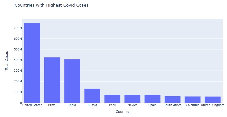
Let’s plot top 10 Total Cases vs Countries
import plotly.express as px
figure = px.bar(data, y=’Total Cases’, x=’Country’,
title=”Countries with Highest Covid Cases”)
figure.show()
Let’s plot top 10 Countries with Highest Deaths
figure = px.bar(data, y=’Total Deaths’, x=’Country’,
title=”Countries with Highest Deaths”)
figure.show()

Let’s compare Total Cases vs Total Deaths for top 10 countries
fig = go.Figure()
fig.add_trace(go.Bar(
x=data[“Country”],
y=data[“Total Cases”],
name=’Total Cases’,
marker_color=’indianred’
))
fig.add_trace(go.Bar(
x=data[“Country”],
y=data[“Total Deaths”],
name=’Total Deaths’,
marker_color=’lightsalmon’
))
fig.update_layout(barmode=’group’, xaxis_tickangle=-45)
fig.show()

let’s plot the Percentage of Total Cases and Deaths
cases = data[“Total Cases”].sum()
deceased = data[“Total Deaths”].sum()
labels = [“Total Cases”, “Total Deaths”]
values = [cases, deceased]
fig = px.pie(data, values=values, names=labels,
title=’Percentage of Total Cases and Deaths’, hole=0.5)
fig.show()

The death rate is given by
death_rate = (data[“Total Deaths”].sum() / data[“Total Cases”].sum()) * 100
print(“Death Rate = “, death_rate)
Death Rate = 3.6144212045653767
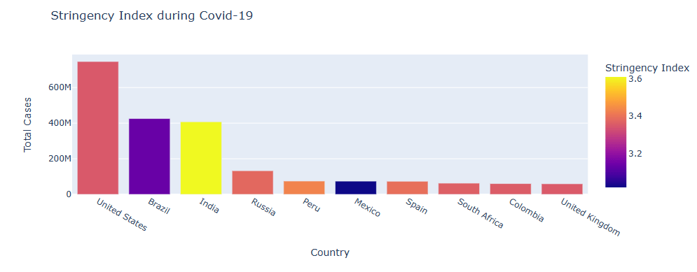
Let’s plot the Stringency Index during COVID-19 for top 10 countries
fig = px.bar(data, x=’Country’, y=’Total Cases’,
hover_data=[‘Population’, ‘Total Deaths’],
color=’Stringency Index’, height=400,
title= “Stringency Index during Covid-19”)
fig.show()
Let’s compare GDP Per Capita Before Covid-19
fig = px.bar(data, x=’Country’, y=’Total Cases’,
hover_data=[‘Population’, ‘Total Deaths’],
color=’GDP Before Covid’, height=400,
title=”GDP Per Capita Before Covid-19″)
fig.show()

Let’s compare GDP Per Capita During Covid-19
fig = px.bar(data, x=’Country’, y=’Total Cases’,
hover_data=[‘Population’, ‘Total Deaths’],
color=’GDP During Covid’, height=400,
title=”GDP Per Capita During Covid-19″)
fig.show()

Let’s compare GDP per Capita before/during COVID-19
fig = go.Figure()
fig.add_trace(go.Bar(
x=data[“Country”],
y=data[“GDP Before Covid”],
name=’GDP Per Capita Before Covid-19′,
marker_color=’indianred’
))
fig.add_trace(go.Bar(
x=data[“Country”],
y=data[“GDP During Covid”],
name=’GDP Per Capita During Covid-19′,
marker_color=’lightsalmon’
))
fig.update_layout(barmode=’group’, xaxis_tickangle=-45)
fig.show()

Let’s plot Human Development Index during Covid-19
fig = px.bar(data, x=’Country’, y=’Total Cases’,
hover_data=[‘Population’, ‘Total Deaths’],
color=’HDI’, height=400,
title=”Human Development Index during Covid-19″)
fig.show()

Vaccine Sentiment Analysis
Finally, let’s turn our attention to the COVID-19 vaccine sentiment analysis.
Let’s set the working directory YOURPATH
import os
os.chdir(‘YOURPATH’)
os. getcwd()
Let’s install and import the key NLP libraries
!pip install nltk
!pip install wordcloud
!pip install statsmodels
import numpy as np # linear algebra
import pandas as pd # data processing, CSV file I/O (e.g. pd.read_csv)
import re
import string
import nltk
import matplotlib.pyplot as plt
import seaborn as sns
sns.set_style(‘darkgrid’)
import plotly.express as ex
import plotly.graph_objs as go
import plotly.offline as pyo
from plotly.subplots import make_subplots
pyo.init_notebook_mode()
nltk.download(‘vader_lexicon’)
from nltk.sentiment.vader import SentimentIntensityAnalyzer as SIA
from wordcloud import WordCloud,STOPWORDS
from pandas.plotting import autocorrelation_plot
from statsmodels.graphics.tsaplots import plot_acf
from statsmodels.graphics.tsaplots import plot_pacf
from statsmodels.tsa.seasonal import seasonal_decompose
from nltk.util import ngrams
from nltk import word_tokenize
from nltk.stem import PorterStemmer
from nltk.stem import WordNetLemmatizer
import random
plt.rc(‘figure’,figsize=(17,13))
Let’s read and edit the input dataset
f_data = pd.read_csv(‘vaccination_tweets.csv’)
f_data.text =f_data.text.str.lower()
Remove twitter handlers
f_data.text = f_data.text.apply(lambda x:re.sub(‘@[^\s]+’,”,x))
Remove hashtags
f_data.text = f_data.text.apply(lambda x:re.sub(r’\B#\S+’,”,x))
Remove URLs
f_data.text = f_data.text.apply(lambda x:re.sub(r”http\S+”, “”, x))
Remove all the special characters
f_data.text = f_data.text.apply(lambda x:’ ‘.join(re.findall(r’\w+’, x)))
Remove all single characters
f_data.text = f_data.text.apply(lambda x:re.sub(r’\s+[a-zA-Z]\s+’, ”, x))
Substituting multiple spaces with single space
f_data.text = f_data.text.apply(lambda x:re.sub(r’\s+’, ‘ ‘, x, flags=re.I))
Let’s invoke SentimentIntensityAnalyzer
sid = SIA()
f_data[‘sentiments’] = f_data[‘text’].apply(lambda x: sid.polarity_scores(‘ ‘.join(re.findall(r’\w+’,x.lower()))))
f_data[‘Positive Sentiment’] = f_data[‘sentiments’].apply(lambda x: x[‘pos’]+1(10-6)) f_data[‘Neutral Sentiment’] = f_data[‘sentiments’].apply(lambda x: x[‘neu’]+1(10-6))
f_data[‘Negative Sentiment’] = f_data[‘sentiments’].apply(lambda x: x[‘neg’]+1(10*-6))
f_data.drop(columns=[‘sentiments’],inplace=True)
Let’s get the f_data info
f_data.shape
(11020, 19)
f_data.info()
<class 'pandas.core.frame.DataFrame'>
RangeIndex: 11020 entries, 0 to 11019
Data columns (total 19 columns):
 #   Column              Non-Null Count  Dtype
---  ------              --------------  -----
 0   id                  11020 non-null  int64
 1   user_name           11020 non-null  object
 2   user_location       8750 non-null   object
 3   user_description    10341 non-null  object
 4   user_created        11020 non-null  object
 5   user_followers      11020 non-null  int64
 6   user_friends        11020 non-null  int64
 7   user_favourites     11020 non-null  int64
 8   user_verified       11020 non-null  bool
 9   date                11020 non-null  object
 10  text                11020 non-null  object
 11  hashtags            8438 non-null   object
 12  source              11019 non-null  object
 13  retweets            11020 non-null  int64
 14  favorites           11020 non-null  int64
 15  is_retweet          11020 non-null  bool
 16  Positive Sentiment  11020 non-null  float64
 17  Neutral Sentiment   11020 non-null  float64
 18  Negative Sentiment  11020 non-null  float64
dtypes: bool(2), float64(3), int64(6), object(8)
memory usage: 1.5+ MB
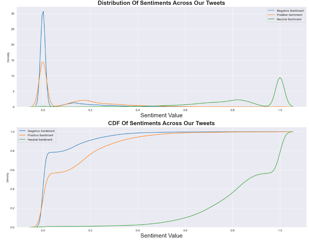
Let’s plot the Distribution and CDF Of Sentiments Across Our Tweets
plt.subplot(2,1,1)
plt.title(‘Distribution Of Sentiments Across Our Tweets’,fontsize=19,fontweight=’bold’)
sns.kdeplot(f_data[‘Negative Sentiment’],bw=0.1)
sns.kdeplot(f_data[‘Positive Sentiment’],bw=0.1)
sns.kdeplot(f_data[‘Neutral Sentiment’],bw=0.1)
plt.legend(labels=[‘Negative Sentiment’, ‘Positive Sentiment’, ‘Neutral Sentiment’])
plt.xlabel(‘Sentiment Value’,fontsize=19)
plt.subplot(2,1,2)
plt.title(‘CDF Of Sentiments Across Our Tweets’,fontsize=19,fontweight=’bold’)
sns.kdeplot(f_data[‘Negative Sentiment’],bw=0.1,cumulative=True)
sns.kdeplot(f_data[‘Positive Sentiment’],bw=0.1,cumulative=True)
sns.kdeplot(f_data[‘Neutral Sentiment’],bw=0.1,cumulative=True)
plt.legend(labels=[‘Negative Sentiment’, ‘Positive Sentiment’, ‘Neutral Sentiment’])
plt.xlabel(‘Sentiment Value’,fontsize=19)
plt.show()
Data Sorting, Feature Engineering and Selecting A Cut-Off For Most Positive/Negative Tweets
f_data = f_data.sort_values(by=’date’)
ft_data=f_data.copy()
ft_data[‘date’] = pd.to_datetime(f_data[‘date’]).dt.date
ft_data[‘year’] = pd.DatetimeIndex(ft_data[‘date’]).year
ft_data[‘month’] = pd.DatetimeIndex(ft_data[‘date’]).month
ft_data[‘day’] = pd.DatetimeIndex(ft_data[‘date’]).day
ft_data[‘day_of_year’] = pd.DatetimeIndex(ft_data[‘date’]).dayofyear
ft_data[‘quarter’] = pd.DatetimeIndex(ft_data[‘date’]).quarter
ft_data[‘season’] = ft_data.month%12 // 3 + 1
plt.subplot(2,1,1)
plt.title(‘Selecting A Cut-Off For Most Positive/Negative Tweets’,fontsize=19,fontweight=’bold’)
ax0 = sns.kdeplot(f_data[‘Negative Sentiment’],bw=0.1)
kde_x, kde_y = ax0.lines[0].get_data()
ax0.fill_between(kde_x, kde_y, where=(kde_x>0.25) ,
interpolate=True, color=’b’)
plt.annotate(‘Cut-Off For Most Negative Tweets’, xy=(0.25, 0.5), xytext=(0.4, 2),
arrowprops=dict(facecolor=’red’, shrink=0.05),fontsize=16,fontweight=’bold’)
ax0.axvline(f_data[‘Negative Sentiment’].mean(), color=’r’, linestyle=’–‘)
ax0.axvline(f_data[‘Negative Sentiment’].median(), color=’tab:orange’, linestyle=’-‘)
plt.legend({‘PDF’:f_data[‘Negative Sentiment’],r’Mean: {:.2f}’.format(f_data[‘Negative Sentiment’].mean()):f_data[‘Negative Sentiment’].mean(),
r’Median: {:.2f}’.format(f_data[‘Negative Sentiment’].median()):f_data[‘Negative Sentiment’].median()})
plt.subplot(2,1,2)
ax1 = sns.kdeplot(f_data[‘Positive Sentiment’],bw=0.1,color=’green’)
plt.annotate(‘Cut-Off For Most Positive Tweets’, xy=(0.4, 0.43), xytext=(0.4, 2),
arrowprops=dict(facecolor=’red’, shrink=0.05),fontsize=16,fontweight=’bold’)
kde_x, kde_y = ax1.lines[0].get_data()
ax1.fill_between(kde_x, kde_y, where=(kde_x>0.4) ,
interpolate=True, color=’green’)
ax1.set_xlabel(‘Sentiment Strength’,fontsize=18)
ax1.axvline(f_data[‘Positive Sentiment’].mean(), color=’r’, linestyle=’–‘)
ax1.axvline(f_data[‘Positive Sentiment’].median(), color=’tab:orange’, linestyle=’-‘)
plt.legend({‘PDF’:f_data[‘Positive Sentiment’],r’Mean: {:.2f}’.format(f_data[‘Positive Sentiment’].mean()):f_data[‘Positive Sentiment’].mean(),
r’Median: {:.2f}’.format(f_data[‘Positive Sentiment’].median()):f_data[‘Positive Sentiment’].median()})
plt.show()

Let’s look at the Common Words Among Most Positive/Negative Tweets
Most_Positive = f_data[f_data[‘Positive Sentiment’].between(0.4,1)]
Most_Negative = f_data[f_data[‘Negative Sentiment’].between(0.25,1)]
Most_Positive_text = ‘ ‘.join(Most_Positive.text)
Most_Negative_text = ‘ ‘.join(Most_Negative.text)
pwc = WordCloud(width=600,height=400,collocations = False).generate(Most_Positive_text)
nwc = WordCloud(width=600,height=400,collocations = False).generate(Most_Negative_text)
plt.subplot(1,2,1)
plt.title(‘Common Words Among Most Positive Tweets’,fontsize=16,fontweight=’bold’)
plt.imshow(pwc)
plt.axis(‘off’)
plt.subplot(1,2,2)
plt.title(‘Common Words Among Most Negative Tweets’,fontsize=16,fontweight=’bold’)
plt.imshow(nwc)
plt.axis(‘off’)
plt.show()

Let’s compare Top 10 Words In Most Positive/Negative Tweets
l_t = Most_Positive_text
w1_dict = dict()
for word in l_t.split():
w= word.strip()
if w in STOPWORDS:
continue
else:
w1_dict[w] = w1_dict.get(w,0)+1
w1_dict = {k: v for k, v in sorted(w1_dict.items(), key=lambda item: item[1],reverse=True)}
l_t = Most_Negative_text
w2_dict = dict()
for word in l_t.split():
w= word.strip()
if w in STOPWORDS:
continue
else:
w2_dict[w] = w2_dict.get(w,0)+1
w2_dict = {k: v for k, v in sorted(w2_dict.items(), key=lambda item: item[1],reverse=True)}
top_10_pos = list(w1_dict.keys())[:10]
top_10_neg = list(w2_dict.keys())[:10]
plt.subplot(1,2,1)
w_c = WordCloud(width=600,height=400,collocations = False,colormap=’nipy_spectral’).generate(‘ ‘.join(top_10_pos))
plt.title(‘Top 10 Words In Most Positive Tweets’,fontsize=19,fontweight=’bold’)
plt.imshow(w_c)
plt.axis(‘off’)
plt.subplot(1,2,2)
w_c = WordCloud(width=600,height=400,collocations = False,colormap=’nipy_spectral’).generate(‘ ‘.join(top_10_neg))
plt.title(‘Top 10 Words In Most Negative Tweets’,fontsize=19,fontweight=’bold’)
plt.imshow(w_c)
plt.axis(‘off’)
plt.show()

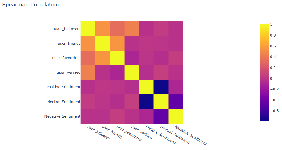
Let’s examine the Spearman correlation matrix
ex.imshow(f_data[[‘user_followers’,’user_friends’,’user_favourites’,’user_verified’,’Positive Sentiment’,
‘Neutral Sentiment’,’Negative Sentiment’]].corr(‘spearman’),title=’Spearman Correlation’)
Conclusions
- We implemented and tested a Python program to get the latest number of confirmed deaths and recovered people of Novel Coronavirus (COVID-19) cases Country/Region – Province/State wise.
- We analyzed the impact of COVID-19 on the global economy using the Kaggle dataset.
- We performed the COVID-19 vaccine sentiment analysis using the Twitter dataset.
Explore More
COVID-19 Geospatial Data Visualization with Plotly, Geopandas, and Folium
50 Coronavirus COVID-19 Free APIs
Interactive Global COVID-19 Data Visualization with Plotly
Comparing 4 Python Libraries for Interactive COVID-19 Data Science Visualization
Embed Socials
https://youtube.com/shorts/F5vSYgIwtAY
Infographic


Make a one-time donation
Make a monthly donation
Make a yearly donation
Choose an amount
Or enter a custom amount
Your contribution is appreciated.
Your contribution is appreciated.
Your contribution is appreciated.

Leave a comment