Featured Photo by Polina Zimmerman on Pexels.

Data Visualization (DV) is the first step towards getting an insight into a large data set in every data science project. DV tools available in Python can be a very effective and efficient way of finding trends, outliers, and hidden patterns in data.

Following the recent DV study and related pilots, our objective is to gain insights that help to contain the coronavirus through charts derived from the COVID-19 dataset. The file contains the cumulative count of confirmed, death and recovered cases of COVID-19 from different countries from 22nd January 2020.

Today we will be comparing the following 4 open-source DV libraries: pyPlot, Plotly, Bokeh, and Vega-Altair.

• pyPlot is a collection of functions that make matplotlib work like MATLAB. This is a comprehensive library for creating static, animated, and interactive visualizations in Python.

• Plotly library makes interactive, publication-quality graphs such as line plots, scatter plots, area charts, bar charts, error bars, box plots, histograms, heatmaps, subplots, multiple-axes, polar charts, and bubble charts.

• Bokeh is a Python library for creating interactive visualizations for modern web browsers. It helps you build beautiful graphics, ranging from simple plots to complex dashboards with streaming datasets. With Bokeh, you can create JavaScript-powered visualizations without writing any JavaScript yourself.
• Vega–Altair is a declarative statistical visualization library for Python, based on Vega and Vega-Lite, and the source is available on GitHub. With Vega-Altair, you can spend more time understanding your data and its meaning. Altair’s API is simple, friendly and consistent and built on top of the powerful Vega-Lite visualization grammar. This elegant simplicity produces beautiful and effective visualizations with a minimal amount of code.

Key Questions:

• How does the Global Spread of the virus look like?
• How intensive the spread of the virus has been in the countries? 
• Does covid19 national lockdowns and self-isolations in different countries have actually impact on COVID19 transmission? 

Libraries

Let’s set the working directory YOURPATH

import os
os.chdir(‘YOURPATH’) # Set working directory
os. getcwd()

Let’s install datapane

!pip install datapane

and import other libraries

import numpy as np
import pandas as pd
import matplotlib.pyplot as plt
import seaborn as sns
pd.set_option(“display.max_columns”,None)
pd.set_option(“display.max_rows”,None)
import warnings
warnings.filterwarnings(“ignore”)
from IPython.display import Image
sns.set(style=”darkgrid”, palette=”pastel”, color_codes=True)
sns.set_context(“paper”)
from datetime import datetime
import datapane as dp

Altair imports

import altair as alt
alt.data_transformers.disable_max_rows()

DataTransformerRegistry.enable('default')

Dataset

Let’s read the input data

df = pd.read_csv(‘covid_19_clean_complete.csv’)
clist = pd.read_csv(‘all_countries.csv’)

df.head()

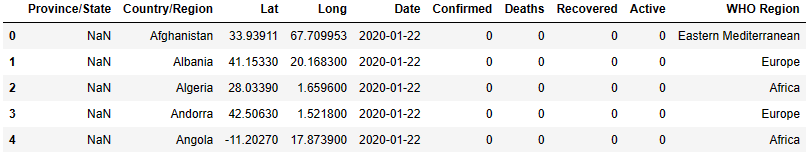
df.shape

(49068, 11)

df.info()

<class 'pandas.core.frame.DataFrame'>
RangeIndex: 49068 entries, 0 to 49067
Data columns (total 11 columns):
 #   Column      Non-Null Count  Dtype         
---  ------      --------------  -----         
 0   state       14664 non-null  object        
 1   country     49068 non-null  object        
 2   lat         49068 non-null  float64       
 3   long        49068 non-null  float64       
 4   date        49068 non-null  datetime64[ns]
 5   confirmed   49068 non-null  int64         
 6   deaths      49068 non-null  int64         
 7   recovered   49068 non-null  int64         
 8   Active      49068 non-null  int64         
 9   WHO Region  49068 non-null  object        
 10  active      49068 non-null  int64         
dtypes: datetime64[ns](1), float64(2), int64(5), object(3)
memory usage: 4.1+ MB

clist.head()

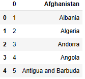
clist.shape

(192, 2)

clist.info()

<class 'pandas.core.frame.DataFrame'>
RangeIndex: 192 entries, 0 to 191
Data columns (total 2 columns):
 #   Column       Non-Null Count  Dtype 
---  ------       --------------  ----- 
 0   0            192 non-null    int64 
 1   Afghanistan  192 non-null    object
dtypes: int64(1), object(1)
memory usage: 3.1+ KB

let’s rename the columns for the sake of convenience
df.rename(columns={‘Date’: ‘date’,
‘Province/State’:’state’,
‘Country/Region’:’country’,
‘Lat’:’lat’, ‘Long’:’long’,
‘Confirmed’: ‘confirmed’,
‘Deaths’:’deaths’,
‘Recovered’:’recovered’
}, inplace=True)

and calculate the difference

Active Case = confirmed – deaths – recovered
df[‘active’] = df[‘confirmed’] – df[‘deaths’] – df[‘recovered’]

We also apply pd.to_datetime to df[‘date’]

df[‘date’] = pd.to_datetime(df[‘date’])

and define the unique country list

country_list = list(df[‘country’].unique())

PyPlot

Let’s plot the ‘confirmed’ column by selecting Germany from country_list

plot = plt.plot(df[‘date’][df[‘country’]==’Germany’], df[‘confirmed’][df[‘country’]==’Germany’])
plt.show()
fig1 = plot

This plot is suitable only for the initial inspection of our dataset.

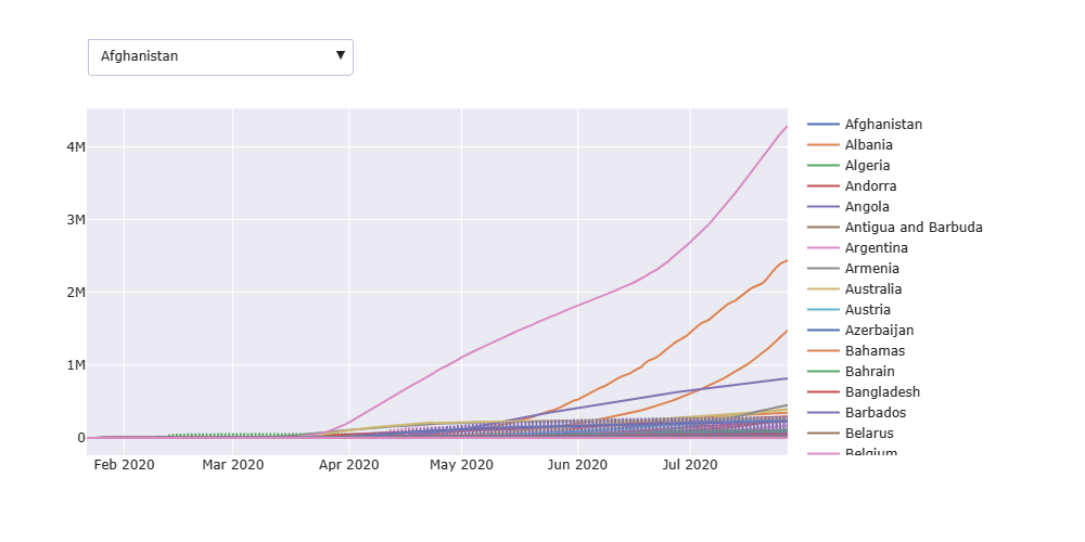
Plotly

Let’s use the Plotly library to plot confirmed COVID-19 cases for all countries

import numpy as np
import pandas as pd
import matplotlib.pyplot as plt
import seaborn as sns
pd.set_option(“display.max_columns”,None)
pd.set_option(“display.max_rows”,None)
import warnings
warnings.filterwarnings(“ignore”)
from IPython.display import Image
sns.set(style=”darkgrid”, palette=”pastel”, color_codes=True)
sns.set_context(“paper”)
from datetime import datetime
import datapane as dp

Plotly imports

import plotly.graph_objects as go
import plotly.express as px
import plotly.io as pio
pio.templates.default = “seaborn”
from plotly.subplots import make_subplots
buttons = []
i = 0

fig3 = go.Figure()

country_list = list(df[‘country’].unique())

for country in country_list:
fig3.add_trace(
go.Scatter(
x = df[‘date’][df[‘country’]==country],
y = df[‘confirmed’][df[‘country’]==country],
name = country, visible = (i==0)
)
)

for country in country_list:
args = [False] * len(country_list)
args[i] = True

#create a button object for the country we are on
button = dict(label = country,
              method = "update",
              args=[{"visible": args}])

#add the button to our list of buttons
buttons.append(button)

#i is an iterable used to tell our "args" list which value to set to True
i+=1

fig3.update_layout(updatemenus=[dict(active=0,
type=”dropdown”,
buttons=buttons,
x = 0,
y = 1.1,
xanchor = ‘left’,
yanchor = ‘bottom’),
])

fig3.update_layout(
autosize=False,
width=1000,
height=500)

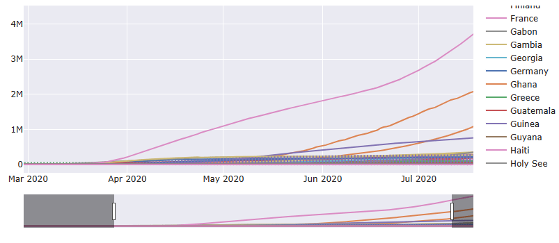
Let’s add the time slider to the above plot

i = 0

fig3 = go.Figure()

country_list = list(df[‘country’].unique())

for country in country_list:
fig3.add_trace(
go.Scatter(
x = df[‘date’][df[‘country’]==country],
y = df[‘confirmed’][df[‘country’]==country],
name = country, visible = (i==0)
)
)

for country in country_list:
args = [False] * len(country_list)
args[i] = True

#create a button object for the country we are on
button = dict(label = country,
              method = "update",
              args=[{"visible": args}])

#add the button to our list of buttons
buttons.append(button)

#i is an iterable used to tell our "args" list which value to set to True
i+=1

fig3.update_layout(updatemenus=[dict(active=0,
type=”dropdown”,
buttons=buttons,
x = 0,
y = 1.1,
xanchor = ‘left’,
yanchor = ‘bottom’),
])

fig3.update_layout(xaxis1_rangeslider_visible=True,
height=600)

fig3.update_layout(
autosize=False,
width=1000,
height=500)

Bokeh

Let’s load the Bokeh notebook

import numpy as np
import pandas as pd
import matplotlib.pyplot as plt
import seaborn as sns
pd.set_option(“display.max_columns”,None)
pd.set_option(“display.max_rows”,None)
import warnings
warnings.filterwarnings(“ignore”)
from IPython.display import Image
sns.set(style=”darkgrid”, palette=”pastel”, color_codes=True)
sns.set_context(“paper”)
from datetime import datetime

import datapane as dp

Bokeh imports:

from bokeh.io import output_file, show, output_notebook, save
from bokeh.models import ColumnDataSource, Select, DateRangeSlider
from bokeh.plotting import figure, show
from bokeh.models import CustomJS
from bokeh.layouts import row,column
output_notebook()

BokehJS 2.4.3 successfully loaded.

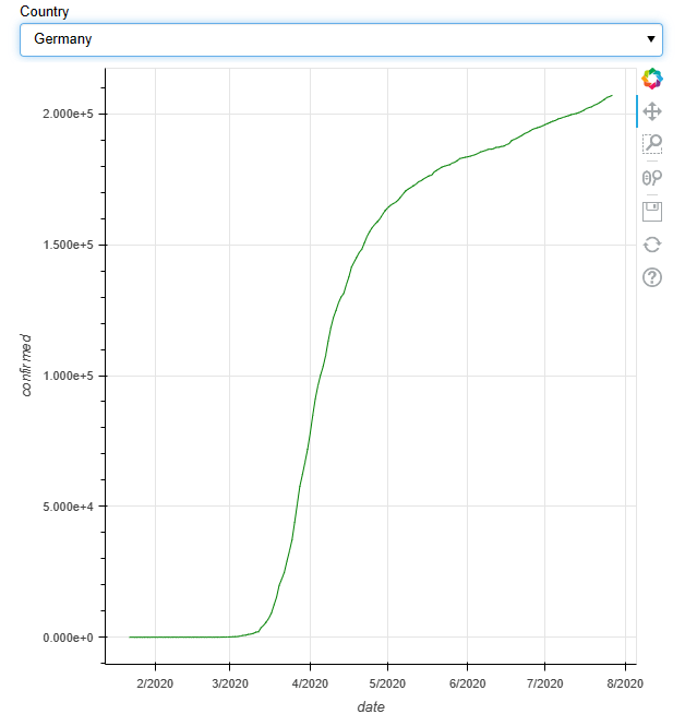
Let’s plot confirmed COVID-19 cases by selecting Germany from the country list

cols1=df.loc[:, [‘country’,’date’, ‘confirmed’]]
cols2 = cols1[cols1[‘country’] == ‘Germany’ ]

Overall = ColumnDataSource(data=cols1)
Curr=ColumnDataSource(data=cols2)

#plot and the menu is linked with each other by this callback function

callback = CustomJS(args=dict(source=Overall, sc=Curr), code=”””
var f = cb_obj.value
sc.data[‘date’]=[]
sc.data[‘confirmed’]=[]
for(var i = 0; i <= source.get_length(); i++){
if (source.data[‘country’][i] == f){
sc.data[‘date’].push(source.data[‘date’][i])
sc.data[‘confirmed’].push(source.data[‘confirmed’][i])
}
}

sc.change.emit();
“””)

menu = Select(options=country_list,value=’Afghanistan’, title = ‘Country’) # drop down menu
bokeh_p=figure(x_axis_label =’date’, y_axis_label = ‘confirmed’, y_axis_type=”linear”,x_axis_type=”datetime”) #creating figure object
bokeh_p.line(x=’date’, y=’confirmed’, color=’green’, source=Curr) # plotting the data using glyph circle
menu.js_on_change(‘value’, callback) # calling the function on change of selection
layout=column(menu, bokeh_p) # creating the layout
show(layout)

Let’s add the time slider to the above plot

cols1=df.loc[:, [‘country’,’date’, ‘confirmed’]]
cols2 = cols1[cols1[‘country’] == ‘Germany’ ]

Overall = ColumnDataSource(data=cols1)
Curr=ColumnDataSource(data=cols2)

#plot and the menu is linked with each other by this callback function

callback = CustomJS(args=dict(source=Overall, sc=Curr), code=”””
var f = cb_obj.value
sc.data[‘date’]=[]
sc.data[‘confirmed’]=[]
for(var i = 0; i <= source.get_length(); i++){
if (source.data[‘country’][i] == f){
sc.data[‘date’].push(source.data[‘date’][i])
sc.data[‘confirmed’].push(source.data[‘confirmed’][i])
}
}

sc.change.emit();
“””)

menu = Select(options=country_list,value=’Afghanistan’, title = ‘Country’) # drop down menu
bokeh_p=figure(x_axis_label =’date’, y_axis_label = ‘confirmed’, y_axis_type=”linear”,x_axis_type=”datetime”) #creating figure object
bokeh_p.line(x=’date’, y=’confirmed’, color=’green’, source=Curr) # plotting the data using glyph circle
menu.js_on_change(‘value’, callback) # calling the function on change of selection

date_range_slider = DateRangeSlider(value=(min(df[‘date’]), max(df[‘date’])),
start=min(df[‘date’]), end=max(df[‘date’]))

date_range_slider.js_link(“value”, bokeh_p.x_range, “start”, attr_selector=0)
date_range_slider.js_link(“value”, bokeh_p.x_range, “end”, attr_selector=1)

layout = column(menu, date_range_slider, bokeh_p)
show(layout) # displaying the layout

Vega-Altair

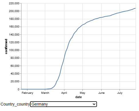
Let’s plot confirmed COVID-19 cases by selecting Germany from the drop-down alt_plot menu

input_dropdown = alt.binding_select(options=country_list)
selection = alt.selection_single(fields=[‘country’], bind=input_dropdown, name=’Country’)

alt_plot = alt.Chart(df).mark_line().encode(
x=’date’,
y=’confirmed’,
tooltip=’confirmed’
).add_selection(
selection
).transform_filter(
selection
)

alt_plot

Let’s add the time slider slider.date[0] to the above plot

input_dropdown = alt.binding_select(options=country_list)
selection = alt.selection_single(fields=[‘country’], bind=input_dropdown, name=’Country’)

def timestamp(t):
return pd.to_datetime(t).timestamp() * 1000

slider = alt.binding_range(
step=30 * 24 * 60 * 60 * 1000, # 30 days in milliseconds
min=timestamp(min(df[‘date’])),
max=timestamp(max(df[‘date’])))

select_date = alt.selection_single(
fields=[‘date’],
bind=slider,
init={‘date’: timestamp(min(df[‘date’]))},
name=’slider’)

alt_plot = alt.Chart(df).mark_line().encode(
x=’date’,
y=’confirmed’,
tooltip=’confirmed’
).add_selection(
selection
).transform_filter(
selection
).add_selection(select_date).transform_filter(
“(year(datum.date) == year(slider.date[0])) && “
“(month(datum.date) == month(slider.date[0]))”
)

alt_plot

Summary

• All 4 libraries can be used to create a plot of COVID-19 cases vs. time (while displaying the date correctly)
• The plt.plot is very useful for the quick initial QC of our dataset prior to EDA.
• We can create a drop-down menu to choose a country with/without time slider, zoom and pan on the plot during EDA
• Bokeh and Vega-Altair have typically been our “go to” for creating interactive COVID-19 plots in Python.
• There are other libraries and nice plotting options to explore in future.

EdTech

COVID19 Data Visualization Using Python

Explore More

Firsthand Data Visualization in R: Examples

What is the Best Interactive Plotting Package in Python?

Visualizing COVID-19 with Pandas & MatPlotLib

Visualizing COVID-19 Data using Julia

Embed Socials