
Featured Photo by @Nate_Dumlao at @unsplash
This post was inspired by the Qullamaggie’s trading journey and its application to the TSLA swing breakouts. Read more about breakouts here.
Our current goal is to extend the above breakout analysis to the $OXY stock.
Motivation
- Occidental Petroleum: The Next Merger Arbitrage Play?
- Protecting Life’s Work: Buffett’s Acquisition Of Occidental Petroleum
- Buffett Buying Occidental: Other Oil Stocks Are More Compelling, Lessons From Buffett’s Railroad Buy
- Occidental Petroleum: Buffett Will Not Get My Shares This Cheap
- Occidental Petroleum among Energy/Material gainers
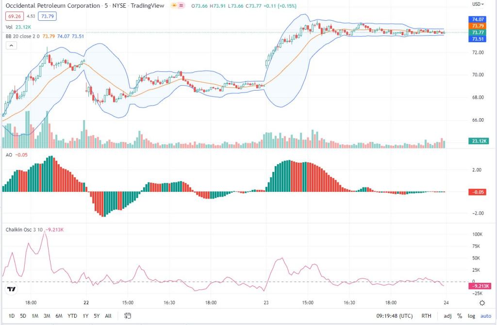
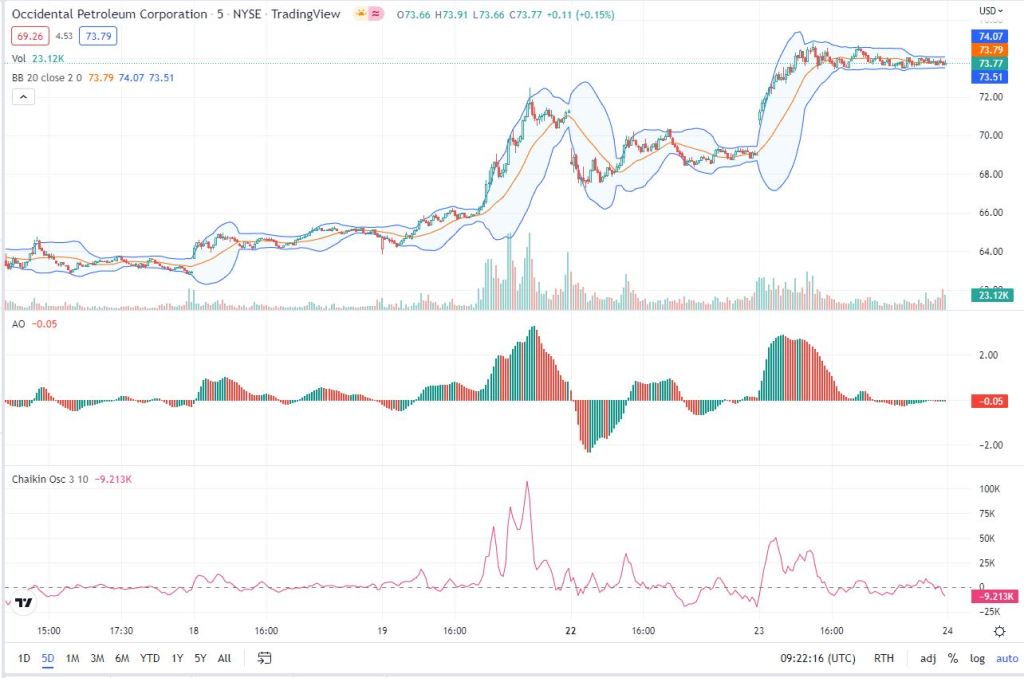
OXY advanced price chart: candlesticks, trading volume, Bollinger bands, Awesome Oscillator (AO), and Chaikin Oscillator.
1D
5D
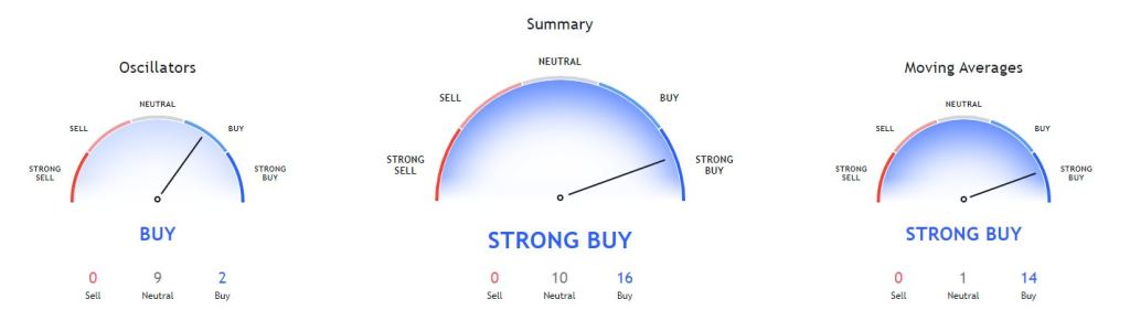
The summary of Occidental Petroleum Corporation is based on the most popular technical indicators, such as Moving Averages, Oscillators and Pivots.
OXY technical analysis
| Name | Value | Action |
|---|---|---|
| Relative Strength Index (14) | 65.42 | Neutral |
| Stochastic %K (14, 3, 3) | 79.62 | Neutral |
| Commodity Channel Index (20) | 165.12 | Neutral |
| Average Directional Index (14) | 33.40 | Neutral |
| Awesome Oscillator | 9.95 | Neutral |
| Momentum (10) | 18.11 | Buy |
| MACD Level (12, 26) | 5.36 | Buy |
| Stochastic RSI Fast (3, 3, 14, 14) | 45.74 | Neutral |
| Williams Percent Range (14) | −5.11 | Neutral |
| Bull Bear Power | 13.54 | Neutral |
| Ultimate Oscillator (7, 14, 28) | 65.77 | Neutral |
| Name | Value | Action |
|---|---|---|
| Exponential Moving Average (10) | 65.43 | Buy |
| Simple Moving Average (10) | 63.40 | Buy |
| Exponential Moving Average (20) | 61.64 | Buy |
| Simple Moving Average (20) | 62.90 | Buy |
| Exponential Moving Average (30) | 57.77 | Buy |
| Simple Moving Average (30) | 58.97 | Buy |
| Exponential Moving Average (50) | 51.24 | Buy |
| Simple Moving Average (50) | 47.96 | Buy |
| Exponential Moving Average (100) | 43.37 | Buy |
| Simple Moving Average (100) | 35.35 | Buy |
| Exponential Moving Average (200) | 43.63 | Buy |
| Simple Moving Average (200) | 38.43 | Buy |
| Ichimoku Base Line (9, 26, 52, 26) | 56.54 | Neutral |
| Volume Weighted Moving Average (20) | 62.64 | Buy |
| Hull Moving Average (9) | 70.74 | Buy |
E2E Workflow
The E2E algorithm is implemented as a sequence of the following steps:
- trend_filter
Take in a pandas series and output a binary array to indicate if a stock
fits the growth criteria (1) or not (0)
Parameters
———-
prices : pd.core.series.Series
The prices we are using to check for growth
growth_4_min : float, optional
The minimum 4 week growth. The default is 25
growth_12_min : float, optional
The minimum 12 week growth. The default is 50
growth_24_min : float, optional
The minimum 24 week growth. The default is 80
Returns
——-
np.array
A binary array showing the positions where the growth criteria is met
- explicit_heat_smooth
Smoothen out a time series using a explicit finite difference method.
Parameters
———-
prices : np.array
The price to smoothen
t_end : float
The time at which to terminate the smootheing (i.e. t = 2)
Returns
——-
P : np.array
The smoothened time-series
Time spacing, must be < 1 for numerical stability
Set up the initial condition
Solve the finite difference scheme for the next time-step
Add the fixed boundary conditions since the above solves the interior points only
- check_consolidation
Smoothen the time-series and check for consolidation, see the
docstring of find_consolidation for the parameters
- find_consolidation
Return a binary array to indicate whether each of the data-points are
classed as consolidating or not
Parameters
———-
prices : np.array
The price time series to check for consolidation
days_to_smooth : int, optional
The length of the time-series to smoothen (days). The default is 50.
perc_change_days : int, optional
The days back to % change compare against (days). The default is 5.
perc_change_thresh : float, optional
The range trading % criteria for consolidation. The default is 0.015.
check_days : int, optional
This says the number of lookback days to check for any consolidation.
If any days in check_days back is consolidating, then the last data
point is said to be consolidating. The default is 5.
Returns
——-
res : np.array
The binary array indicating consolidation (1) or not (0)
- We download the Yahoofinance $OXY data and call the above functions
- Data visualizations using matplotlib scatter plot – original Close price + Volume size (red) vs breakouts (green).
Results
Set working directory YOURPATH
import os
os.chdir(‘YOURPATH’)
os. getcwd()
Import libraries
import numpy as np
import pandas as pd
import yfinance as yf
Define functions
def trend_filter(prices: pd.core.series.Series,
growth_4_min: float = 25.,
growth_12_min: float = 50.,
growth_24_min: float = 80.) -> np.array:
”’
Take in a pandas series and output a binary array to indicate if a stock
fits the growth criteria (1) or not (0)
Parameters
———-
prices : pd.core.series.Series
The prices we are using to check for growth
growth_4_min : float, optional
The minimum 4 week growth. The default is 25
growth_12_min : float, optional
The minimum 12 week growth. The default is 50
growth_24_min : float, optional
The minimum 24 week growth. The default is 80
Returns
——-
np.array
A binary array showing the positions where the growth criteria is met
”’
growth_func = lambda x: 100*(x.values[-1]/x.min() - 1)

growth_4 = df['Close'].rolling(20).apply(growth_func) > growth_4_min
growth_12 = df['Close'].rolling(60).apply(growth_func) > growth_12_min
growth_24 = df['Close'].rolling(120).apply(growth_func) > growth_24_min

return np.where(
    growth_4 | growth_12 | growth_24,
    1,
    0,
)
if name == ‘main‘:
df = yf.download('OXY')
df.loc[:, 'trend_filter'] = trend_filter(df['Close'])
df.dropna()
[*********************100%***********************] 1 of 1 completed
df_trending = df[df[‘trend_filter’] == 1]
def explicit_heat_smooth(prices: np.array,
t_end: float = 5.0) -> np.array:
”’
Smoothen out a time series using a explicit finite difference method.
Parameters
———-
prices : np.array
The price to smoothen
t_end : float
The time at which to terminate the smootheing (i.e. t = 2)
Returns
——-
P : np.array
The smoothened time-series
”’
k = 0.1 # Time spacing, must be < 1 for numerical stability

# Set up the initial condition
P = prices

t = 0
while t < t_end:
    # Solve the finite difference scheme for the next time-step
    P = k*(P[2:] + P[:-2]) + P[1:-1]*(1-2*k)

    # Add the fixed boundary conditions since the above solves the interior
    # points only
    P = np.hstack((
        np.array([prices[0]]),
        P,
        np.array([prices[-1]]),
    ))
    t += k

return P
def check_consolidation(prices: np.array,
perc_change_days: int,
perc_change_thresh: float,
check_days: int) -> int:
”’
Smoothen the time-series and check for consolidation, see the
docstring of find_consolidation for the parameters
”’
# Find the smoothed representation of the time series
prices = explicit_heat_smooth(prices)

# Perc change of the smoothed time series to perc_change_days days prior
perc_change = prices[perc_change_days:]/prices[:-perc_change_days] - 1

consolidating = np.where(np.abs(perc_change) < perc_change_thresh, 1, 0)

# Provided one entry in the last n days passes the consolidation check,
# we say that the financial instrument is in consolidation on the end day
if np.sum(consolidating[-check_days:]) > 0:
    return 1
else:
    return 0
def find_consolidation(prices: np.array,
days_to_smooth: int = 50,
perc_change_days: int = 5,
perc_change_thresh: float = 0.015,
check_days: int = 5) -> np.array:
”’
Return a binary array to indicate whether each of the data-points are
classed as consolidating or not
Parameters
———-
prices : np.array
The price time series to check for consolidation
days_to_smooth : int, optional
The length of the time-series to smoothen (days). The default is 50.
perc_change_days : int, optional
The days back to % change compare against (days). The default is 5.
perc_change_thresh : float, optional
The range trading % criteria for consolidation. The default is 0.015.
check_days : int, optional
This says the number of lookback days to check for any consolidation.
If any days in check_days back is consolidating, then the last data
point is said to be consolidating. The default is 5.
Returns
——-
res : np.array
The binary array indicating consolidation (1) or not (0)
”’
res = np.full(prices.shape, np.nan)

for idx in range(days_to_smooth, prices.shape[0]):
    res[idx] = check_consolidation(
        prices = prices[idx-days_to_smooth:idx],
        perc_change_days = perc_change_days,
        perc_change_thresh = perc_change_thresh,
        check_days = check_days,
    )

return res
Let’s proceed with main
if name == ‘main‘:
df = yf.download('TSLA')
df.loc[:, 'consolidating'] = find_consolidation(df['Close'].values)
df.dropna()
[*********************100%***********************] 1 of 1 completed
df = yf.download(‘TSLA’)
df.loc[:, ‘consolidating’] = find_consolidation(df[‘Close’].values)
df.loc[:, ‘trend_filter’] = trend_filter(df[‘Close’])
df.loc[:, ‘filtered’] = np.where(
df[‘consolidating’] + df[‘trend_filter’] == 2,
True,
False,
)
[*********************100%***********************] 1 of 1 completed
Our dataframe df looks as follows
<class 'pandas.core.frame.DataFrame'>
DatetimeIndex: 3051 entries, 2010-06-29 to 2022-08-10
Data columns (total 9 columns):
 #   Column         Non-Null Count  Dtype
---  ------         --------------  -----
 0   Open           3051 non-null   float64
 1   High           3051 non-null   float64
 2   Low            3051 non-null   float64
 3   Close          3051 non-null   float64
 4   Adj Close      3051 non-null   float64
 5   Volume         3051 non-null   int64
 6   consolidating  3001 non-null   float64
 7   trend_filter   3051 non-null   int32
 8   filtered       3051 non-null   bool
dtypes: bool(1), float64(6), int32(1), int64(1)
memory usage: 205.6 KB
import numpy as np
import seaborn as sns
import matplotlib.pyplot as plt
import pandas as pd
df.index = pd.DatetimeIndex(data=df.index, tz=’US/Eastern’)
import matplotlib
plt.figure(figsize=(12,10))
matplotlib.rcParams.update({‘font.size’: 18})
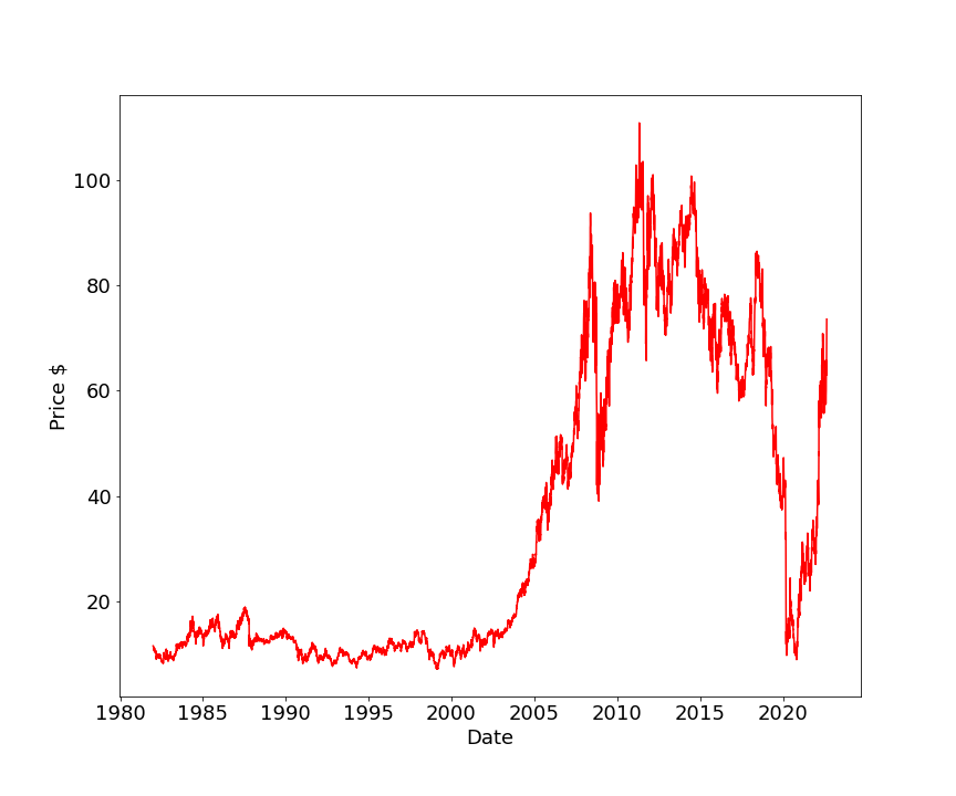
import matplotlib.pyplot as plt
plt.plot(dft.DateTime,df.Close, ‘r’)
plt.xlabel(“Date”)
plt.ylabel(“Price $”)
plt.savefig(‘tslaprice.png’)
plt.figure(figsize=(12,10))
scal=5e5
plt.scatter(df0.index, df0[“Close”],color=’red’,s=df0[“Volume”]/scal,alpha=0.4)
plt.scatter(df1.index, df1[“Close”],color=’green’,s=df1[“Volume”]/scal,alpha=0.4)
plt.xlabel(“Date”)
plt.ylabel(“Price $”)
plt.legend([“Close” , “Filtered”], facecolor=’bisque’,
loc=’upper center’, bbox_to_anchor=(0.5, -0.08),
ncol=2)
plt.grid()
plt.show()
plt.savefig(‘oxypriceswingfilter.png’)

Conclusions
print(df.loc[‘2021-01-01 00:00:00-04:00′:’2022-08-22 00:00:00-04:00’])
                    Adj Close    Volume  consolidating  trend_filter  \
Date
2021-01-04 00:00:00-05:00  17.351271  18497800            0.0             1
2021-01-05 00:00:00-05:00  19.101311  37293800            1.0             1
2021-01-06 00:00:00-05:00  19.886841  37156400            1.0             1
2021-01-07 00:00:00-05:00  20.453615  24299300            1.0             1
2021-01-08 00:00:00-05:00  19.966389  18277900            0.0             1
...                              ...       ...            ...           ...
2022-08-16 00:00:00-04:00  63.509998  16662200            1.0             0
2022-08-17 00:00:00-04:00  62.970001  14889800            1.0             0
2022-08-18 00:00:00-04:00  64.879997  16818000            1.0             0
2022-08-19 00:00:00-04:00  71.290001  79840900            0.0             0
2022-08-22 00:00:00-04:00  69.029999  47888500            0.0             0

                           filtered
Date
2021-01-04 00:00:00-05:00     False
2021-01-05 00:00:00-05:00      True
2021-01-06 00:00:00-05:00      True
2021-01-07 00:00:00-05:00      True
2021-01-08 00:00:00-05:00     False
...                             ...
2022-08-16 00:00:00-04:00     False
2022-08-17 00:00:00-04:00     False
2022-08-18 00:00:00-04:00     False
2022-08-19 00:00:00-04:00     False
2022-08-22 00:00:00-04:00     False
We focus on the “True” trading signals and ignore “False”.
The above scatter plot and the table help identify the setups. You need to have a watchlist ready before the market open. You should also probably have alerts set, and know how many shares you want to buy.
A swing trader can use the daily chart to find these setups, but it also works on the weekly chart and the intraday (1- and 5-minute) charts.
Read More
QULLAMAGGIE
OXY Stock Update Wednesday, 25 May 2022
OXY Stock Analysis, Thursday, 23 June 2022
Track All Markets with TradingView
Predicting Trend Reversal in Algorithmic Trading using Stochastic Oscillator in Python
S&P 500 Algorithmic Trading with FBProphet


Leave a comment