The goal of the here presented pilot study is to develop and test an end-to-end Python-3 script in Jupyter that implements algorithmic trading (aka automated trading, black-box trading, or algo-trading). Thanks to high-level automation and integration of multiple tasks, the script can simultaneously analyze hundreds of technical indicators, run simulations and forecasts, perform real-time technical analysis and generate trading signals and alerts at a speed and frequency that is impossible for a human trader.

Trading Technical Indicators (tti) is an open source Python library for Technical Analysis of trading indicators within the realm of Algorithmic Trading, using traditional methods and machine learning algorithms.
PyPI TTI – this is where Traditional Technical Analysis and AI are met:
- Calculate technical indicators (62 indicators supported).
- Produce graphs for any technical indicator.
- Get trading signals for each indicator.
- Trading simulation based on trading signals.
- Machine Learning integration for prices prediction.
Let’s begin with the Monte Carlo simulation to find the best data fit and predict future stock prices.
Let’s import the relevant libraries
import numpy as np
from datetime import datetime
import pandas_datareader as pdr
from scipy.stats import norm
Let’s define some parameters
days_to_test = 30 #Days for our best fit test
days_to_predict = 1 #How many days in the future we want to go
simulations = 1000 #How many simulations to run
ticker = ‘BAC’ #Our stock ticker name
Bank of America Corp is our stock of interest.
Let’s read the historical stock data from Yahoo Finance
data = pdr.get_data_yahoo([ticker],
start=datetime(1990, 1, 1),
end=datetime.today().strftime(‘%Y-%m-%d’))[‘Close’]
Let’s calculate several key parameters
daily_return = np.log(1 + data[ticker].pct_change())
average_daily_return = daily_return.mean()
variance = daily_return.var()
drift = average_daily_return – (variance/2)
standard_deviation = daily_return.std()
and make predictions
predictions = np.zeros(days_to_test+days_to_predict)
predictions[0] = data[ticker][-days_to_test]
pred_collection = np.ndarray(shape=(simulations,days_to_test+days_to_predict))
for j in range(0,simulations):
for i in range(1,days_to_test+days_to_predict):
random_value = standard_deviation * norm.ppf(np.random.rand())
predictions[i] = predictions[i-1] * np.exp(drift + random_value)
pred_collection[j] = predictions
differences = np.array([])
for k in range(0,simulations):
difference_arrays = np.subtract(data[ticker].values[-days_to_test:],pred_collection[k][:-1])
difference_values = np.sum(np.abs(difference_arrays))
differences = np.append(differences,difference_values)
best_fit = np.argmin(differences)
future_price = pred_collection[best_fit][-1]
type(future_price)
numpy.float64
print(future_price)
31.845747517762227
print(predictions)
[37.45000076 37.27929377 36.76698951 35.60097048 35.43851925 34.00310714
 33.55056974 32.5020387  32.17673994 32.40621735 31.96776456 32.07664156
 33.27317133 33.49117672 31.69846963 33.4838012  36.3412071  35.703381
 35.55212438 35.384061   34.26848077 35.62129531 35.02340644 33.75911575
 34.37497056 34.79596405 33.18222406 32.12827983 31.67886237 31.50734121
 30.4862908 ]
print(predictions.shape)
(31,)
print(data.shape)
(8180, 1)
dataraw=data[ticker].values[-(days_to_test+days_to_predict):]
print(dataraw.shape)
(31,)
Let’s plot predictions and raw data
from matplotlib import pyplot as plt
from matplotlib.pyplot import figure
figure(figsize=(8, 6), dpi=80)
plt.plot(dataraw,label=’Raw Data’,linewidth=2)
plt.plot(predictions,label=’Predicted Data’,linewidth=2)
plt.xlabel(“Days”)
plt.ylabel(“Price”)
plt.legend()

print(dataraw[30])
31.920000076293945
We can see that the difference between predictions and raw data is only 0.25%
Let’s plot the historical data
plt.plot(data,linewidth=2)

Next, we will look at the available trading indicators and the tti.indicators usage examples.
Let’s install the TTI library
!pip install tti
Let’s begin with the A/D indicator
from tti.indicators import AccumulationDistributionLine
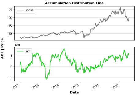
The accumulation/distribution indicator (A/D) is a cumulative indicator that uses volume and price to assess whether a stock is being accumulated or distributed. The A/D measure seeks to identify divergences between the stock price and the volume flow. This provides insight into how strong a trend is. If the price is rising but the indicator is falling, then it suggests that buying or accumulation volume may not be enough to support the price rise and a price decline could be forthcoming.
Let’s import the relevant libraries
import pandas as pd
import datetime
import numpy as np
import matplotlib.pyplot as plt
from pandas.plotting import scatter_matrix
!pip install yfinance
import yfinance as yf
%matplotlib inline
Let’s consider the following Indian stocks as an example
start = “2017-01-01”
end = ‘2022-6-17’
tcs = yf.download(‘TCS’,start,end)
infy = yf.download(‘INFY’,start,end)
wipro = yf.download(‘WIPRO.NS’,start,end)
[*********************100%***********************]  1 of 1 completed
[*********************100%***********************]  1 of 1 completed
[*********************100%***********************]  1 of 1 completed
TCS = Tata Consultancy Services Limited
INFY = Infosys Ltd
WIPRO = Wipro Limited
Let’s select INFY as an example
df=infy
adl_indicator = AccumulationDistributionLine(input_data=df)
Get indicator’s calculated data
print(‘\nTechnical Indicator data:\n’, adl_indicator.getTiData())
echnical Indicator data:
                   adl
Date
2017-01-03    1220076
2017-01-04    7429572
2017-01-05    5938753
2017-01-06   27622113
2017-01-09   38246447
...               ...
2022-06-10  107633755
2022-06-13  104228143
2022-06-14  110571789
2022-06-15  124032379
2022-06-16  122503296

[1374 rows x 1 columns]
Get indicator’s value for a specific date
print(‘\nTechnical Indicator value at 2022-06-16:’, adl_indicator.getTiValue(‘2022-06-16’))
Technical Indicator value at 2022-06-16: [122503296]
Get the most recent indicator’s value
print(‘\nMost recent Technical Indicator value:’, adl_indicator.getTiValue())
Most recent Technical Indicator value: [122503296]
Get signal from indicator
print(‘\nTechnical Indicator signal:’, adl_indicator.getTiSignal())
Technical Indicator signal: ('buy', -1)
Show the Graph for the calculated Technical Indicator
adl_indicator.getTiGraph().show()
Save the Graph for the calculated Technical Indicator
adl_indicator.getTiGraph().savefig(‘../TTI/example_AccumulationDistributionLine.png’)
print(‘\nGraph for the calculated ADL indicator data, saved.’)
Graph for the calculated ADL indicator data, saved.
Execute simulation based on trading signals
simulation_data, simulation_statistics, simulation_graph = \
adl_indicator.getTiSimulation(
close_values=df[[‘close’]], max_exposure=None,
short_exposure_factor=1.5)
print(‘\nSimulation Data:\n’, simulation_data)
print(‘\nSimulation Statistics:\n’, simulation_statistics)
Save the Graph for the executed trading signal simulation
simulation_graph.savefig(‘../TTI/simulation_AccumulationDistributionLine.png’)
print(‘\nGraph for the executed trading signal simulation, saved.’)
Simulation Data:
            signal open_trading_action stock_value     exposure  \
Date
2017-01-03   hold                none        7.37          0.0
2017-01-04    buy                long       7.565        7.565
2017-01-05    buy                long        7.51       15.075
2017-01-06    buy                long        7.41       22.485
2017-01-09    buy                long        7.48       22.555
...           ...                 ...         ...          ...
2022-06-10    buy                long       18.33  1399.507497
2022-06-13    buy                long       17.85  1417.357497
2022-06-14    buy                long       18.24  1417.747497
2022-06-15    buy                long   18.290001  1417.797498
2022-06-16    buy                long       17.67  1435.467498

           portfolio_value    earnings     balance
Date
2017-01-03             0.0         0.0         0.0
2017-01-04           7.565         0.0       7.565
2017-01-05           15.02         0.0       15.02
2017-01-06           22.23         0.0       22.23
2017-01-09           22.44        0.07       22.51
...                    ...         ...         ...
2022-06-10     -384.929998  199.284986 -185.645012
2022-06-13     -357.000008  199.284986 -157.715022
2022-06-14     -364.799995  199.674985  -165.12501
2022-06-15     -365.800018  199.724987 -166.075032
2022-06-16     -335.730001  199.724987 -136.005015

[1374 rows x 7 columns]
Simulation Statistics:
 {'number_of_trading_days': 1374, 'number_of_buy_signals': 955, 'number_of_ignored_buy_signals': 0, 'number_of_sell_signals': 392, 'number_of_ignored_sell_signals': 0, 'last_stock_value': 17.67, 'last_exposure': 1435.47, 'last_open_long_positions': 29, 'last_open_short_positions': 48, 'last_portfolio_value': -335.73, 'last_earnings': 199.72, 'final_balance': -136.01}

Graph for the executed trading signal simulation, saved.

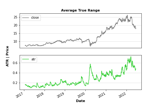
We Can Calculate the Average True Range (ATR) Easy with Pandas DataFrames. This is an important volatility indicator.
For example, consider $NFLX since 2020-1-1
import numpy as np
import pandas_datareader as pdr
import datetime as dt
start = dt.datetime(2020, 1, 1)
data = pdr.get_data_yahoo(“NFLX”, start)
high_low = data[‘High’] – data[‘Low’]
high_close = np.abs(data[‘High’] – data[‘Close’].shift())
low_close = np.abs(data[‘Low’] – data[‘Close’].shift())
ranges = pd.concat([high_low, high_close, low_close], axis=1)
true_range = np.max(ranges, axis=1)
atr = true_range.rolling(14).sum()/14
The ATR plot (blue curve) vs the original stock price (orange curve) is as follows
import matplotlib.pyplot as plt
fig, ax = plt.subplots()
atr.plot(ax=ax)
data[‘Close’].plot(ax=ax, secondary_y=True, alpha=0.3)
plt.show()

Let’s see how ATR can be computed using TTI by considering $INFY
from tti.indicators import AverageTrueRange
atr_indicator = AverageTrueRange(input_data=df)
Get indicator’s value for a specific date
print(‘\nTechnical Indicator value at 2022-06-16:’, atr_indicator.getTiValue(‘2022-06-16’))
Get the most recent indicator’s value
print(‘\nMost recent Technical Indicator value:’, atr_indicator.getTiValue())
Get signal from indicator
print(‘\nTechnical Indicator signal:’, atr_indicator.getTiSignal())
Show the Graph for the calculated Technical Indicator
atr_indicator.getTiGraph().show()
Save the Graph for the calculated Technical Indicator
atr_indicator.getTiGraph().savefig(‘../TTI/example_ATR.png’)
print(‘\nGraph for the calculated ATR indicator data, saved.’)
Technical Indicator value at 2022-06-16: [0.4831]

Most recent Technical Indicator value: [0.4831]

Technical Indicator signal: ('buy', -1)
Graph for the calculated ATR indicator data, saved.
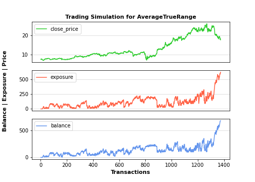
Execute simulation based on trading signals
simulation_data, simulation_statistics, simulation_graph = \
atr_indicator.getTiSimulation(
close_values=df[[‘close’]], max_exposure=None,
short_exposure_factor=1.5)
print(‘\nSimulation Data:\n’, simulation_data)
print(‘\nSimulation Statistics:\n’, simulation_statistics)
Save the Graph for the executed trading signal simulation
simulation_graph.savefig(‘../TTI/simulation_ATR.png’)
print(‘\nGraph for the executed trading signal simulation, saved.’)
Simulation Data:
            signal open_trading_action stock_value    exposure portfolio_value  \
Date
2017-01-03   hold                none        7.37         0.0             0.0
2017-01-04   hold                none       7.565         0.0             0.0
2017-01-05   hold                none        7.51         0.0             0.0
2017-01-06   hold                none        7.41         0.0             0.0
2017-01-09   hold                none        7.48         0.0             0.0
...           ...                 ...         ...         ...             ...
2022-06-10    buy                long       18.33  587.754999      458.249998
2022-06-13    buy                long       17.85  605.604999       464.10001
2022-06-14    buy                long       18.24  605.994998      474.239994
2022-06-15    buy                long   18.290001     606.045      475.540024
2022-06-16    buy                long       17.67     623.715      477.090002

              earnings     balance
Date
2017-01-03         0.0         0.0
2017-01-04         0.0         0.0
2017-01-05         0.0         0.0
2017-01-06         0.0         0.0
2017-01-09         0.0         0.0
...                ...         ...
2022-06-10  207.524981  665.774979
2022-06-13  207.524981  671.624991
2022-06-14   207.91498  682.154974
2022-06-15  207.964982  683.505005
2022-06-16  207.964982  685.054984

[1374 rows x 7 columns]
Simulation Statistics:
 {'number_of_trading_days': 1374, 'number_of_buy_signals': 1289, 'number_of_ignored_buy_signals': 0, 'number_of_sell_signals': 71, 'number_of_ignored_sell_signals': 0, 'last_stock_value': 17.67, 'last_exposure': 623.71, 'last_open_long_positions': 28, 'last_open_short_positions': 1, 'last_portfolio_value': 477.09, 'last_earnings': 207.96, 'final_balance': 685.05}

Graph for the executed trading signal simulation, saved.
Recall that the average true range (ATR) is a market volatility indicator used in technical analysis. It is typically derived from the 14-day simple moving average of a series of true range indicators. The ATR was originally developed for use in commodities markets but has since been applied to all types of securities.
Let’s look at the Bollinger Bands (BB) to Gauge Trends. These bands are a trading tool used to determine entry and exit points for a trade.
from tti.indicators import BollingerBands
bb_indicator = BollingerBands(input_data=df)
Get indicator’s value for a specific date
print(‘\nTechnical Indicator value at 2022-06-15:’, bb_indicator.getTiValue(‘2022-06-15’))
Get the most recent indicator’s value
print(‘\nMost recent Technical Indicator value:’, bb_indicator.getTiValue())
Get signal from indicator
print(‘\nTechnical Indicator signal:’, bb_indicator.getTiSignal())
Show the Graph for the calculated Technical Indicator
bb_indicator.getTiGraph().show()
Save the Graph for the calculated Technical Indicator
bb_indicator.getTiGraph().savefig(‘../TTI/example_BB.png’)
print(‘\nGraph for the calculated BB indicator data, saved.’)
Technical Indicator value at 2022-06-15: [18.7665, 19.6881, 17.8449]

Most recent Technical Indicator value: [18.711, 19.749, 17.673]

Technical Indicator signal: ('buy', -1)
Graph for the calculated BB indicator data, saved.

Execute simulation based on trading signals
simulation_data, simulation_statistics, simulation_graph = \
bb_indicator.getTiSimulation(
close_values=df[[‘close’]], max_exposure=None,
short_exposure_factor=1.5)
print(‘\nSimulation Data:\n’, simulation_data)
print(‘\nSimulation Statistics:\n’, simulation_statistics)
Save the Graph for the executed trading signal simulation
simulation_graph.savefig(‘../TTI/simulation_BB.png’)
print(‘\nGraph for the executed trading signal simulation, saved.’)
Simulation Data:
            signal open_trading_action stock_value    exposure portfolio_value  \
Date
2017-01-03   hold                none        7.37         0.0             0.0
2017-01-04   hold                none       7.565         0.0             0.0
2017-01-05   hold                none        7.51         0.0             0.0
2017-01-06   hold                none        7.41         0.0             0.0
2017-01-09   hold                none        7.48         0.0             0.0
...           ...                 ...         ...         ...             ...
2022-06-10   hold                none       18.33  206.519999          -36.66
2022-06-13    buy                long       17.85  224.369999          -17.85
2022-06-14   hold                none       18.24  206.519999          -36.48
2022-06-15   hold                none   18.290001  206.519999      -36.580002
2022-06-16    buy                long       17.67  224.189999          -17.67

             earnings    balance
Date
2017-01-03        0.0        0.0
2017-01-04        0.0        0.0
2017-01-05        0.0        0.0
2017-01-06        0.0        0.0
2017-01-09        0.0        0.0
...               ...        ...
2022-06-10  24.760002 -11.899998
2022-06-13  24.760002   6.910001
2022-06-14  25.150001 -11.329998
2022-06-15  25.150001 -11.430001
2022-06-16  25.150001   7.480001

[1374 rows x 7 columns]

Simulation Statistics:
 {'number_of_trading_days': 1374, 'number_of_buy_signals': 65, 'number_of_ignored_buy_signals': 0, 'number_of_sell_signals': 106, 'number_of_ignored_sell_signals': 0, 'last_stock_value': 17.67, 'last_exposure': 224.19, 'last_open_long_positions': 5, 'last_open_short_positions': 6, 'last_portfolio_value': -17.67, 'last_earnings': 25.15, 'final_balance': 7.48}

Graph for the executed trading signal simulation, saved.

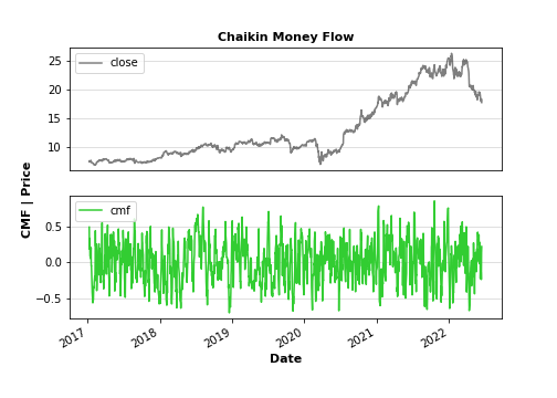
The Chaikin Money Flow (CMF) is an indicator created by Marc Chaikin in the 1980s to monitor the accumulation and distribution of a stock over a specified period. The default CMF period is 21 days. The indicator readings range between +1 and -1.
Get indicator’s value for a specific date
print(‘\nTechnical Indicator value at 2022-06-15:’, cmf_indicator.getTiValue(‘2022-06-15’))
Get the most recent indicator’s value
print(‘\nMost recent Technical Indicator value:’, cmf_indicator.getTiValue())
Get signal from indicator
print(‘\nTechnical Indicator signal:’, cmf_indicator.getTiSignal())
Show the Graph for the calculated Technical Indicator
cmf_indicator.getTiGraph().show()
Save the Graph for the calculated Technical Indicator
cmf_indicator.getTiGraph().savefig(‘../TTI/example_CMF.png’)
print(‘\nGraph for the calculated CMF indicator data, saved.’)
Execute simulation based on trading signals
simulation_data, simulation_statistics, simulation_graph = \
cmf_indicator.getTiSimulation(
close_values=df[[‘close’]], max_exposure=None,
short_exposure_factor=1.5)
print(‘\nSimulation Data:\n’, simulation_data)
print(‘\nSimulation Statistics:\n’, simulation_statistics)
Save the Graph for the executed trading signal simulation
simulation_graph.savefig(‘../TTI/simulation_CMF.png’)
print(‘\nGraph for the executed trading signal simulation, saved.’)
Technical Indicator value at 2022-06-15: [0.1354]

Most recent Technical Indicator value: [0.2206]

Technical Indicator signal: ('buy', -1)
Graph for the calculated CMF indicator data, saved.

Simulation Data:
            signal open_trading_action stock_value    exposure portfolio_value  \
Date
2017-01-03   hold                none        7.37         0.0             0.0
2017-01-04   hold                none       7.565         0.0             0.0
2017-01-05   hold                none        7.51         0.0             0.0
2017-01-06   hold                none        7.41         0.0             0.0
2017-01-09   hold                none        7.48         0.0             0.0
...           ...                 ...         ...         ...             ...
2022-06-10    buy                long       18.33  260.900001          -54.99
2022-06-13    buy                long       17.85  278.750001      -35.700001
2022-06-14   hold                none       18.24  260.900001      -54.719999
2022-06-15   hold                none   18.290001  260.900001      -54.870003
2022-06-16    buy                long       17.67  278.570001          -35.34

             earnings    balance
Date
2017-01-03        0.0        0.0
2017-01-04        0.0        0.0
2017-01-05        0.0        0.0
2017-01-06        0.0        0.0
2017-01-09        0.0        0.0
...               ...        ...
2022-06-10  55.725003   0.735003
2022-06-13  55.725003  20.025002
2022-06-14  56.115003   1.395003
2022-06-15  56.115003      1.245
2022-06-16  56.115003  20.775002

[1374 rows x 7 columns]

Simulation Statistics:
 {'number_of_trading_days': 1374, 'number_of_buy_signals': 160, 'number_of_ignored_buy_signals': 0, 'number_of_sell_signals': 218, 'number_of_ignored_sell_signals': 0, 'last_stock_value': 17.67, 'last_exposure': 278.57, 'last_open_long_positions': 6, 'last_open_short_positions': 8, 'last_portfolio_value': -35.34, 'last_earnings': 56.12, 'final_balance': 20.78}

Graph for the executed trading signal simulation, saved.

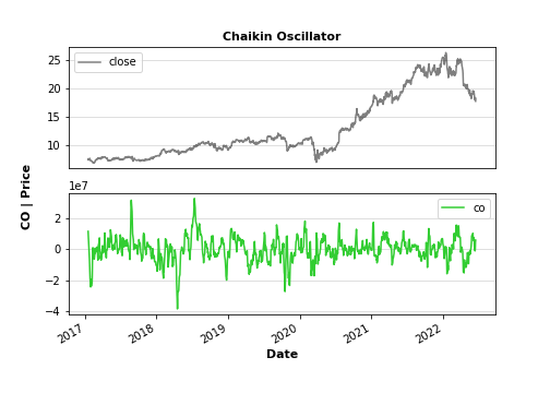
Let’s look at the Chaikin Oscillator. The Chaikin Oscillator (CO) is the difference between the 3-day and 10-day EMAs of the A/D Line discussed above. Like other momentum indicators, this indicator is designed to anticipate directional changes in the A/D Line by measuring the momentum behind the movements. A momentum change is the first step to a trend change. Anticipating trend changes in the A/D Line can help chartists anticipate trend changes in the underlying security. The CO generates signals with crosses above/below the zero line or with bullish/bearish divergences.
from tti.indicators import ChaikinOscillator
co_indicator = ChaikinOscillator(input_data=df)
Get indicator’s value for a specific date
print(‘\nTechnical Indicator value at 2022-06-15:’, co_indicator.getTiValue(‘2022-06-15’))
Get the most recent indicator’s value
print(‘\nMost recent Technical Indicator value:’, co_indicator.getTiValue())
Get signal from indicator
print(‘\nTechnical Indicator signal:’, co_indicator.getTiSignal())
Show the Graph for the calculated Technical Indicator
co_indicator.getTiGraph().show()
Save the Graph for the calculated Technical Indicator
co_indicator.getTiGraph().savefig(‘../TTI/example_CO.png’)
print(‘\nGraph for the calculated CO indicator data, saved.’)
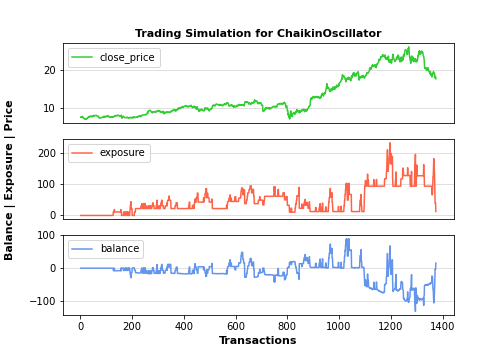
Execute simulation based on trading signals
simulation_data, simulation_statistics, simulation_graph = \
co_indicator.getTiSimulation(
close_values=df[[‘close’]], max_exposure=None,
short_exposure_factor=1.5)
print(‘\nSimulation Data:\n’, simulation_data)
print(‘\nSimulation Statistics:\n’, simulation_statistics)
Save the Graph for the executed trading signal simulation
simulation_graph.savefig(‘../TTI/simulation_CO.png’)
print(‘\nGraph for the executed trading signal simulation, saved.’)
Technical Indicator value at 2022-06-15: [4952520.5672]

Most recent Technical Indicator value: [5958499.6774]

Technical Indicator signal: ('hold', 0)
Graph for the calculated CO indicator data, saved.

Simulation Data:
            signal open_trading_action stock_value   exposure portfolio_value  \
Date
2017-01-03   hold                none        7.37        0.0             0.0
2017-01-04   hold                none       7.565        0.0             0.0
2017-01-05   hold                none        7.51        0.0             0.0
2017-01-06   hold                none        7.41        0.0             0.0
2017-01-09   hold                none        7.48        0.0             0.0
...           ...                 ...         ...        ...             ...
2022-06-10   sell               short       18.33  93.449999          -73.32
2022-06-13   hold                none       17.85     39.135      -35.700001
2022-06-14   hold                none       18.24     39.135          -36.48
2022-06-15   hold                none   18.290001     39.135      -36.580002
2022-06-16   hold                none       17.67     12.375          -17.67

             earnings    balance
Date
2017-01-03        0.0        0.0
2017-01-04        0.0        0.0
2017-01-05        0.0        0.0
2017-01-06        0.0        0.0
2017-01-09        0.0        0.0
...               ...        ...
2022-06-10  32.400006 -40.919994
2022-06-13  32.910004  -2.789997
2022-06-14  32.910004  -3.569995
2022-06-15  32.910004  -3.669998
2022-06-16  33.080004  15.410004

[1374 rows x 7 columns]

Simulation Statistics:
 {'number_of_trading_days': 1374, 'number_of_buy_signals': 162, 'number_of_ignored_buy_signals': 0, 'number_of_sell_signals': 74, 'number_of_ignored_sell_signals': 0, 'last_stock_value': 17.67, 'last_exposure': 12.38, 'last_open_long_positions': 0, 'last_open_short_positions': 1, 'last_portfolio_value': -17.67, 'last_earnings': 33.08, 'final_balance': 15.41}

Graph for the executed trading signal simulation, saved.
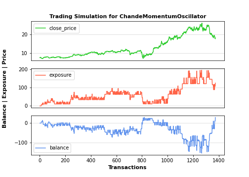
The Chande momentum oscillator (CMO) is a technical indicator that uses momentum to identify relative strength or weakness in a market:
- The chosen time frame greatly affects signals generated by the indicator.
- Pattern recognition often generates more reliable signals than absolute oscillator levels.
- Overbought-oversold indicators are less effective in strongly trending markets.
from tti.indicators import ChandeMomentumOscillator
cmo_indicator = ChandeMomentumOscillator(input_data=df)
Get indicator’s value for a specific date
print(‘\nTechnical Indicator value at 2022-06-15:’, cmo_indicator.getTiValue(‘2022-06-15’))
Get the most recent indicator’s value
print(‘\nMost recent Technical Indicator value:’, cmo_indicator.getTiValue())
Get signal from indicator
print(‘\nTechnical Indicator signal:’, cmo_indicator.getTiSignal())
Show the Graph for the calculated Technical Indicator
cmo_indicator.getTiGraph().show()
Save the Graph for the calculated Technical Indicator
cmo_indicator.getTiGraph().savefig(‘../TTI/example_CMO.png’)
print(‘\nGraph for the calculated CMO indicator data, saved.’)
Execute simulation based on trading signals
simulation_data, simulation_statistics, simulation_graph = \
cmo_indicator.getTiSimulation(
close_values=df[[‘close’]], max_exposure=None,
short_exposure_factor=1.5)
print(‘\nSimulation Data:\n’, simulation_data)
print(‘\nSimulation Statistics:\n’, simulation_statistics)
Save the Graph for the executed trading signal simulation
simulation_graph.savefig(‘../TTI/simulation_CMO.png’)
print(‘\nGraph for the executed trading signal simulation, saved.’)
Technical Indicator value at 2022-06-15: [-49.7142]

Most recent Technical Indicator value: [-57.8947]

Technical Indicator signal: ('buy', -1)

Graph for the calculated CMO indicator data, saved.

Simulation Data:
            signal open_trading_action stock_value    exposure portfolio_value  \
Date
2017-01-03   hold                none        7.37         0.0             0.0
2017-01-04   hold                none       7.565         0.0             0.0
2017-01-05   hold                none        7.51         0.0             0.0
2017-01-06   hold                none        7.41         0.0             0.0
2017-01-09   hold                none        7.48         0.0             0.0
...           ...                 ...         ...         ...             ...
2022-06-10   hold                none       18.33  107.789999          -18.33
2022-06-13   hold                none       17.85  107.789999          -17.85
2022-06-14   hold                none       18.24  107.789999          -18.24
2022-06-15   hold                none   18.290001  107.789999      -18.290001
2022-06-16    buy                long       17.67  125.459999             0.0

             earnings    balance
Date
2017-01-03        0.0        0.0
2017-01-04        0.0        0.0
2017-01-05        0.0        0.0
2017-01-06        0.0        0.0
2017-01-09        0.0        0.0
...               ...        ...
2022-06-10  29.255002  10.925003
2022-06-13  29.255002  11.405002
2022-06-14  29.255002  11.015003
2022-06-15  29.255002  10.965002
2022-06-16  29.255002  29.255002

[1374 rows x 7 columns]

Simulation Statistics:
 {'number_of_trading_days': 1374, 'number_of_buy_signals': 76, 'number_of_ignored_buy_signals': 0, 'number_of_sell_signals': 121, 'number_of_ignored_sell_signals': 0, 'last_stock_value': 17.67, 'last_exposure': 125.46, 'last_open_long_positions': 3, 'last_open_short_positions': 3, 'last_portfolio_value': 0.0, 'last_earnings': 29.26, 'final_balance': 29.26}

Graph for the executed trading signal simulation, saved.
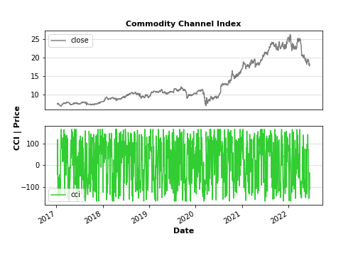
The Commodity Channel Index (CCI) is a technical indicator that measures the difference between the current price and the historical average price. When the CCI is above zero, it indicates the price is above the historic average. Conversely, when the CCI is below zero, the price is below the historic average.
from tti.indicators import CommodityChannelIndex
cci_indicator = CommodityChannelIndex(input_data=df)
Get indicator’s value for a specific date
print(‘\nTechnical Indicator value at 2022-06-15:’, cci_indicator.getTiValue(‘2022-06-15’))
Get the most recent indicator’s value
print(‘\nMost recent Technical Indicator value:’, cci_indicator.getTiValue())
Get signal from indicator
print(‘\nTechnical Indicator signal:’, cci_indicator.getTiSignal())
Show the Graph for the calculated Technical Indicator
cci_indicator.getTiGraph().show()
Save the Graph for the calculated Technical Indicator
cci_indicator.getTiGraph().savefig(‘../TTI/example_CCI.png’)
print(‘\nGraph for the calculated CCI indicator data, saved.’)
Execute simulation based on trading signals
simulation_data, simulation_statistics, simulation_graph = \
cci_indicator.getTiSimulation(
close_values=df[[‘close’]], max_exposure=None,
short_exposure_factor=1.5)
print(‘\nSimulation Data:\n’, simulation_data)
print(‘\nSimulation Statistics:\n’, simulation_statistics)
Save the Graph for the executed trading signal simulation
simulation_graph.savefig(‘../TTI/simulation_CCI.png’)
print(‘\nGraph for the executed trading signal simulation, saved.’)
Technical Indicator value at 2022-06-15: [-34.6475]

Most recent Technical Indicator value: [-112.9162]

Technical Indicator signal: ('buy', -1)
Graph for the calculated CCI indicator data, saved.

Simulation Data:
            signal open_trading_action stock_value    exposure portfolio_value  \
Date
2017-01-03   hold                none        7.37         0.0             0.0
2017-01-04   hold                none       7.565         0.0             0.0
2017-01-05   hold                none        7.51         0.0             0.0
2017-01-06   hold                none        7.41         0.0             0.0
2017-01-09   hold                none        7.48         0.0             0.0
...           ...                 ...         ...         ...             ...
2022-06-10    buy                long       18.33  334.484997           54.99
2022-06-13    buy                long       17.85  352.334997       71.400002
2022-06-14   hold                none       18.24  334.484997       54.719999
2022-06-15   hold                none   18.290001  334.484997       54.870003
2022-06-16    buy                long       17.67  352.154997           70.68

             earnings     balance
Date
2017-01-03        0.0         0.0
2017-01-04        0.0         0.0
2017-01-05        0.0         0.0
2017-01-06        0.0         0.0
2017-01-09        0.0         0.0
...               ...         ...
2022-06-10  76.254998  131.244998
2022-06-13  76.254998     147.655
2022-06-14  76.644998  131.364997
2022-06-15  76.644998     131.515
2022-06-16  76.644998  147.324998

[1374 rows x 7 columns]

Simulation Statistics:
 {'number_of_trading_days': 1374, 'number_of_buy_signals': 198, 'number_of_ignored_buy_signals': 0, 'number_of_sell_signals': 282, 'number_of_ignored_sell_signals': 0, 'last_stock_value': 17.67, 'last_exposure': 352.15, 'last_open_long_positions': 11, 'last_open_short_positions': 7, 'last_portfolio_value': 70.68, 'last_earnings': 76.64, 'final_balance': 147.32}

Graph for the executed trading signal simulation, saved.

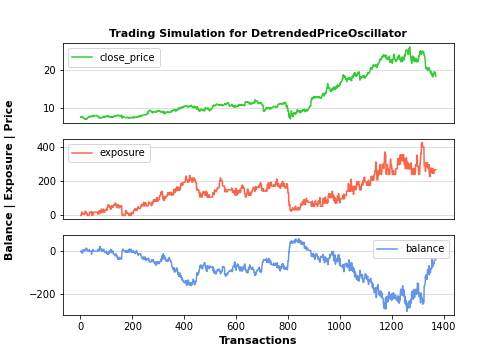
The detrended price oscillator (DPO) is an indicator in technical analysis that attempts to eliminate the long-term trends in prices by using a displaced moving average so it does not react to the most current price action. This allows the indicator to show intermediate overbought and oversold levels effectively.
from tti.indicators import DetrendedPriceOscillator
dpo_indicator = DetrendedPriceOscillator(input_data=df)
Get indicator’s value for a specific date
print(‘\nTechnical Indicator value at 2022-06-15:’, dpo_indicator.getTiValue(‘2022-06-15’))
Get the most recent indicator’s value
print(‘\nMost recent Technical Indicator value:’, dpo_indicator.getTiValue())
Get signal from indicator
print(‘\nTechnical Indicator signal:’, dpo_indicator.getTiSignal())
Show the Graph for the calculated Technical Indicator
dpo_indicator.getTiGraph().show()
Save the Graph for the calculated Technical Indicator
dpo_indicator.getTiGraph().savefig(‘../TTI/example_DPO.png’)
print(‘\nGraph for the calculated DPO indicator data, saved.’)
Execute simulation based on trading signals
simulation_data, simulation_statistics, simulation_graph = \
dpo_indicator.getTiSimulation(
close_values=df[[‘close’]], max_exposure=None,
short_exposure_factor=1.5)
print(‘\nSimulation Data:\n’, simulation_data)
print(‘\nSimulation Statistics:\n’, simulation_statistics)
Save the Graph for the executed trading signal simulation
simulation_graph.savefig(‘../TTI/simulation_DPO.png’)
print(‘\nGraph for the executed trading signal simulation, saved.’)
Technical Indicator value at 2022-06-15: None

Most recent Technical Indicator value: [0.12]

Technical Indicator signal: ('hold', 0)

Graph for the calculated DPO indicator data, saved.

Simulation Data:
            signal open_trading_action stock_value exposure portfolio_value  \
Date
2017-01-03   hold                none        7.37      0.0             0.0
2017-01-04   hold                none       7.565      0.0             0.0
2017-01-05   hold                none        7.51      0.0             0.0
2017-01-06   sell               short        7.41   11.115           -7.41
2017-01-09    buy                long        7.48   18.595             0.0
...           ...                 ...         ...      ...             ...
2022-06-10   hold                none       18.33   264.75          -91.65
2022-06-13    NaN                 NaN         NaN      NaN             NaN
2022-06-14    NaN                 NaN         NaN      NaN             NaN
2022-06-15    NaN                 NaN         NaN      NaN             NaN
2022-06-16    NaN                 NaN         NaN      NaN             NaN

             earnings    balance
Date
2017-01-03        0.0        0.0
2017-01-04        0.0        0.0
2017-01-05        0.0        0.0
2017-01-06        0.0      -7.41
2017-01-09        0.0        0.0
...               ...        ...
2022-06-10  55.260003 -36.389997
2022-06-13        NaN        NaN
2022-06-14        NaN        NaN
2022-06-15        NaN        NaN
2022-06-16        NaN        NaN

[1374 rows x 7 columns]

Simulation Statistics:
 {'number_of_trading_days': 1370, 'number_of_buy_signals': 224, 'number_of_ignored_buy_signals': 0, 'number_of_sell_signals': 226, 'number_of_ignored_sell_signals': 0, 'last_stock_value': 18.33, 'last_exposure': 264.75, 'last_open_long_positions': 4, 'last_open_short_positions': 9, 'last_portfolio_value': -91.65, 'last_earnings': 55.26, 'final_balance': -36.39}

Graph for the executed trading signal simulation, saved.
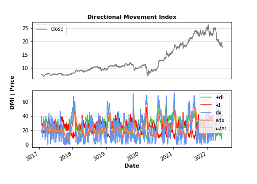
Let’s look at the indicator that identifies in which direction the price of an asset is moving:
- The directional movement index (DMI) is a technical indicator that measures both the strength and direction of a price movement and is intended to reduce false signals.
- The DMI utilizes two standard indicators, one negative (-DM) and one positive (+DN), in conjunction with a third, the average directional index (ADX), which is non-directional but shows momentum.
- The larger the spread between the two primary lines, the stronger the price trend. If +DI is way above -DI the price trend is strongly up. If -DI is way above +DI then the price trend is strongly down.
- ADX measures the strength of the trend, either up or down; a reading above 25 indicates a strong trend.
from tti.indicators import DirectionalMovementIndex
dmi_indicator = DirectionalMovementIndex(input_data=df)
Get indicator’s value for a specific date
print(‘\nTechnical Indicator value at 2022-06-15:’, dmi_indicator.getTiValue(‘2022-06-15’))
Get the most recent indicator’s value
print(‘\nMost recent Technical Indicator value:’, dmi_indicator.getTiValue())
Get signal from indicator
print(‘\nTechnical Indicator signal:’, dmi_indicator.getTiSignal())
Show the Graph for the calculated Technical Indicator
dmi_indicator.getTiGraph().show()
Save the Graph for the calculated Technical Indicator
dmi_indicator.getTiGraph().savefig(‘../TTI/example_dmi.png’)
print(‘\nGraph for the calculated dmi indicator data, saved.’)
Execute simulation based on trading signals
simulation_data, simulation_statistics, simulation_graph = \
dmi_indicator.getTiSimulation(
close_values=df[[‘close’]], max_exposure=None,
short_exposure_factor=1.5)
print(‘\nSimulation Data:\n’, simulation_data)
print(‘\nSimulation Statistics:\n’, simulation_statistics)
Save the Graph for the executed trading signal simulation
simulation_graph.savefig(‘../TTI/simulation_dmi.png’)
print(‘\nGraph for the executed trading signal simulation, saved.’)
Technical Indicator value at 2022-06-15: [18.2314, 38.9129, 36.1917, 31.9486, 36.8952]

Most recent Technical Indicator value: [16.3714, 39.3787, 41.2687, 32.6143, 36.6857]

Technical Indicator signal: ('hold', 0)
Graph for the calculated dmi indicator data, saved.

Simulation Data:
            signal open_trading_action stock_value   exposure portfolio_value  \
Date
2017-01-03   hold                none        7.37        0.0             0.0
2017-01-04   hold                none       7.565        0.0             0.0
2017-01-05   hold                none        7.51        0.0             0.0
2017-01-06   hold                none        7.41        0.0             0.0
2017-01-09   hold                none        7.48        0.0             0.0
...           ...                 ...         ...        ...             ...
2022-06-10   hold                none       18.33  37.649999          -36.66
2022-06-13   hold                none       17.85  37.649999      -35.700001
2022-06-14   hold                none       18.24  37.649999          -36.48
2022-06-15   hold                none   18.290001  37.649999      -36.580002
2022-06-16   hold                none       17.67  37.649999          -35.34

            earnings    balance
Date
2017-01-03       0.0        0.0
2017-01-04       0.0        0.0
2017-01-05       0.0        0.0
2017-01-06       0.0        0.0
2017-01-09       0.0        0.0
...              ...        ...
2022-06-10  8.490003 -28.169997
2022-06-13  8.490003 -27.209998
2022-06-14  8.490003 -27.989996
2022-06-15  8.490003 -28.089999
2022-06-16  8.490003 -26.849997

[1374 rows x 7 columns]

Simulation Statistics:
 {'number_of_trading_days': 1374, 'number_of_buy_signals': 27, 'number_of_ignored_buy_signals': 0, 'number_of_sell_signals': 30, 'number_of_ignored_sell_signals': 0, 'last_stock_value': 17.67, 'last_exposure': 37.65, 'last_open_long_positions': 0, 'last_open_short_positions': 2, 'last_portfolio_value': -35.34, 'last_earnings': 8.49, 'final_balance': -26.85}

Graph for the executed trading signal simulation, saved.

Let’s look at the double exponential moving average (DEMA). This is a technical indicator that was devised to reduce the lag in the results produced by a traditional moving average. Technical traders use it to lessen the amount of “noise” that can distort the movements on a price chart:
from tti.indicators import DoubleExponentialMovingAverage
dema_indicator = DoubleExponentialMovingAverage(input_data=df)
Get indicator’s value for a specific date
print(‘\nTechnical Indicator value at 2022-06-15:’, dema_indicator.getTiValue(‘2022-06-15’))
Get the most recent indicator’s value
print(‘\nMost recent Technical Indicator value:’, dema_indicator.getTiValue())
Get signal from indicator
print(‘\nTechnical Indicator signal:’, dema_indicator.getTiSignal())
Show the Graph for the calculated Technical Indicator
dema_indicator.getTiGraph().show()
Save the Graph for the calculated Technical Indicator
dema_indicator.getTiGraph().savefig(‘../TTI/example_dema.png’)
print(‘\nGraph for the calculated dema indicator data, saved.’)
Execute simulation based on trading signals
simulation_data, simulation_statistics, simulation_graph = \
dema_indicator.getTiSimulation(
close_values=df[[‘close’]], max_exposure=None,
short_exposure_factor=1.5)
print(‘\nSimulation Data:\n’, simulation_data)
print(‘\nSimulation Statistics:\n’, simulation_statistics)
Save the Graph for the executed trading signal simulation
simulation_graph.savefig(‘../TTI/simulation_dema.png’)
print(‘\nGraph for the executed trading signal simulation, saved.’)
Technical Indicator value at 2022-06-15: [18.1512]

Most recent Technical Indicator value: [17.8323]

Technical Indicator signal: ('buy', -1)

Graph for the calculated dema indicator data, saved.

Simulation Data:
            signal open_trading_action stock_value    exposure portfolio_value  \
Date
2017-01-03   hold                none        7.37         0.0             0.0
2017-01-04   hold                none       7.565         0.0             0.0
2017-01-05   hold                none        7.51         0.0             0.0
2017-01-06   hold                none        7.41         0.0             0.0
2017-01-09   hold                none        7.48         0.0             0.0
...           ...                 ...         ...         ...             ...
2022-06-10    buy                long       18.33  437.709995      366.599998
2022-06-13    buy                long       17.85  455.559996      374.850008
2022-06-14   hold                none       18.24  437.709995      364.799995
2022-06-15   hold                none   18.290001  437.709995      365.800018
2022-06-16    buy                long       17.67  455.379995      371.070002

              earnings     balance
Date
2017-01-03         0.0         0.0
2017-01-04         0.0         0.0
2017-01-05         0.0         0.0
2017-01-06         0.0         0.0
2017-01-09         0.0         0.0
...                ...         ...
2022-06-10  100.444993  467.044991
2022-06-13  100.444993  475.295001
2022-06-14  100.834992  465.634988
2022-06-15  100.834992  466.635011
2022-06-16  100.834992  471.904994

[1374 rows x 7 columns]

Simulation Statistics:
 {'number_of_trading_days': 1374, 'number_of_buy_signals': 672, 'number_of_ignored_buy_signals': 0, 'number_of_sell_signals': 0, 'number_of_ignored_sell_signals': 0, 'last_stock_value': 17.67, 'last_exposure': 455.38, 'last_open_long_positions': 21, 'last_open_short_positions': 0, 'last_portfolio_value': 371.07, 'last_earnings': 100.83, 'final_balance': 471.9}

Graph for the executed trading signal simulation, saved.

Let’s look at the Ease of Movement indicator that shows the relationship between price and volume, and it’s often used to assess the strength of an underlying trend:
- Ease of Movement calculates how easily a price can move up or down.
- The calculation subtracts yesterday’s average price from today’s average price and divides the difference by volume.
from tti.indicators import EaseOfMovement
eom_indicator = EaseOfMovement(input_data=df,period=1, fill_missing_values=False)
Get indicator’s value for a specific date
print(‘\nTechnical Indicator value at 2022-06-15:’, eom_indicator.getTiValue(‘2022-06-15’))
Get the most recent indicator’s value
print(‘\nMost recent Technical Indicator value:’, eom_indicator.getTiValue())
Get signal from indicator
print(‘\nTechnical Indicator signal:’, eom_indicator.getTiSignal())
Show the Graph for the calculated Technical Indicator
eom_indicator.getTiGraph().show()
Save the Graph for the calculated Technical Indicator
eom_indicator.getTiGraph().savefig(‘../TTI/example_eom.png’)
print(‘\nGraph for the calculated eom indicator data, saved.’)
Execute simulation based on trading signals
simulation_data, simulation_statistics, simulation_graph = \
eom_indicator.getTiSimulation(
close_values=df[[‘close’]], max_exposure=None,
short_exposure_factor=1.5)
print(‘\nSimulation Data:\n’, simulation_data)
print(‘\nSimulation Statistics:\n’, simulation_statistics)
Save the Graph for the executed trading signal simulation
simulation_graph.savefig(‘../TTI/simulation_eom.png’)
print(‘\nGraph for the executed trading signal simulation, saved.’)
Technical Indicator value at 2022-06-15: [-0.0, -0.0]

Most recent Technical Indicator value: [-0.0001, -0.0001]

Technical Indicator signal: ('hold', 0)

Graph for the calculated eom indicator data, saved.

Simulation Data:
            signal open_trading_action stock_value    exposure portfolio_value  \
Date
2017-01-03   hold                none        7.37         0.0             0.0
2017-01-04   hold                none       7.565         0.0             0.0
2017-01-05   hold                none        7.51         0.0             0.0
2017-01-06   hold                none        7.41         0.0             0.0
2017-01-09   hold                none        7.48         0.0             0.0
...           ...                 ...         ...         ...             ...
2022-06-10   hold                none       18.33  131.235002             0.0
2022-06-13   hold                none       17.85  131.235002             0.0
2022-06-14    buy                long       18.24  149.475002           18.24
2022-06-15   hold                none   18.290001  131.235002             0.0
2022-06-16   hold                none       17.67  131.235002             0.0

             earnings    balance
Date
2017-01-03        0.0        0.0
2017-01-04        0.0        0.0
2017-01-05        0.0        0.0
2017-01-06        0.0        0.0
2017-01-09        0.0        0.0
...               ...        ...
2022-06-10      23.25      23.25
2022-06-13      23.25      23.25
2022-06-14      23.25      41.49
2022-06-15  23.300001  23.300001
2022-06-16  23.300001  23.300001

[1374 rows x 7 columns]

Simulation Statistics:
 {'number_of_trading_days': 1374, 'number_of_buy_signals': 41, 'number_of_ignored_buy_signals': 0, 'number_of_sell_signals': 39, 'number_of_ignored_sell_signals': 0, 'last_stock_value': 17.67, 'last_exposure': 131.24, 'last_open_long_positions': 3, 'last_open_short_positions': 3, 'last_portfolio_value': 0.0, 'last_earnings': 23.3, 'final_balance': 23.3}

Graph for the executed trading signal simulation, saved.

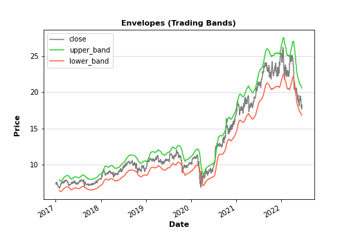
Let’s look at the Envelopes (ENV) indicator. ENV is a tool that attempts to identify the upper and lower bands of a trading range. It does this by plotting two moving average envelopes on a price chart, one shifted up to a certain distance above the price and the other shifted below.
from tti.indicators import Envelopes
env_indicator = Envelopes(input_data=df)
Get indicator’s value for a specific date
print(‘\nTechnical Indicator value at 2022-06-15:’, env_indicator.getTiValue(‘2022-06-15’))
Get the most recent indicator’s value
print(‘\nMost recent Technical Indicator value:’, env_indicator.getTiValue())
Get signal from indicator
print(‘\nTechnical Indicator signal:’, env_indicator.getTiSignal())
Show the Graph for the calculated Technical Indicator
env_indicator.getTiGraph().show()
Save the Graph for the calculated Technical Indicator
env_indicator.getTiGraph().savefig(‘../TTI/example_env.png’)
print(‘\nGraph for the calculated env indicator data, saved.’)
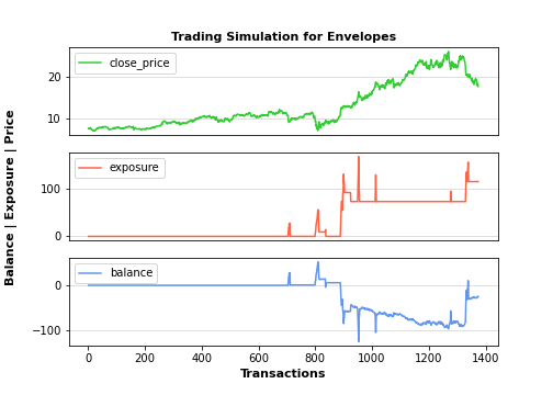
Execute simulation based on trading signals
simulation_data, simulation_statistics, simulation_graph = \
env_indicator.getTiSimulation(
close_values=df[[‘close’]], max_exposure=None,
short_exposure_factor=1.5)
print(‘\nSimulation Data:\n’, simulation_data)
print(‘\nSimulation Statistics:\n’, simulation_statistics)
Save the Graph for the executed trading signal simulation
simulation_graph.savefig(‘../TTI/simulation_env.png’)
print(‘\nGraph for the executed trading signal simulation, saved.’)
Technical Indicator value at 2022-06-15: [20.6431, 16.8898]

Most recent Technical Indicator value: [20.5821, 16.8399]

Technical Indicator signal: ('hold', 0)
Graph for the calculated env indicator data, saved.

Simulation Data:
            signal open_trading_action stock_value    exposure portfolio_value  \
Date
2017-01-03   hold                none        7.37         0.0             0.0
2017-01-04   hold                none       7.565         0.0             0.0
2017-01-05   hold                none        7.51         0.0             0.0
2017-01-06   hold                none        7.41         0.0             0.0
2017-01-09   hold                none        7.48         0.0             0.0
...           ...                 ...         ...         ...             ...
2022-06-10   hold                none       18.33  114.934999          -36.66
2022-06-13   hold                none       17.85  114.934999      -35.700001
2022-06-14   hold                none       18.24  114.934999          -36.48
2022-06-15   hold                none   18.290001  114.934999      -36.580002
2022-06-16   hold                none       17.67  114.934999          -35.34

           earnings    balance
Date
2017-01-03      0.0        0.0
2017-01-04      0.0        0.0
2017-01-05      0.0        0.0
2017-01-06      0.0        0.0
2017-01-09      0.0        0.0
...             ...        ...
2022-06-10    10.68     -25.98
2022-06-13    10.68     -25.02
2022-06-14    10.68 -25.799999
2022-06-15    10.68 -25.900002
2022-06-16    10.68     -24.66

[1374 rows x 7 columns]

Simulation Statistics:
 {'number_of_trading_days': 1374, 'number_of_buy_signals': 28, 'number_of_ignored_buy_signals': 0, 'number_of_sell_signals': 19, 'number_of_ignored_sell_signals': 0, 'last_stock_value': 17.67, 'last_exposure': 114.93, 'last_open_long_positions': 2, 'last_open_short_positions': 4, 'last_portfolio_value': -35.34, 'last_earnings': 10.68, 'final_balance': -24.66}

Graph for the executed trading signal simulation, saved.
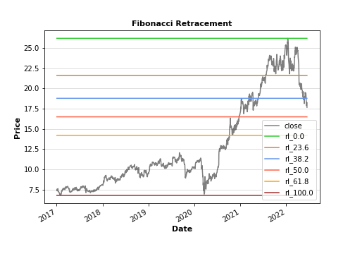
In finance, Fibonacci retracement is a method of technical analysis for determining support and resistance levels. It is named after the Fibonacci sequence of numbers, whose ratios provide price levels to which markets tend to retrace a portion of a move, before a trend continues in the original direction.
Fibonacci retracement levels—stemming from the Fibonacci sequence—are horizontal lines that indicate where support and resistance are likely to occur.
Each level is associated with a percentage. The percentage is how much of a prior move the price has retraced. The Fibonacci retracement levels are 23.6%, 38.2%, 61.8%, and 78.6%. While not officially a Fibonacci ratio, 50% is also used.
The indicator is useful because it can be drawn between any two significant price points, such as a high and a low. The indicator will then create the levels between those two points.
Suppose the price of a stock rises $10 and then drops $2.36. In that case, it has retraced 23.6%, which is a Fibonacci number. Fibonacci numbers are found throughout nature. Therefore, many traders believe that these numbers also have relevance in financial markets:
from tti.indicators import FibonacciRetracement
fr_indicator = FibonacciRetracement(input_data=df)
Get indicator’s value for a specific date
print(‘\nTechnical Indicator value at 2022-06-15:’, fr_indicator.getTiValue(‘2022-06-15’))
Get the most recent indicator’s value
print(‘\nMost recent Technical Indicator value:’, fr_indicator.getTiValue())
Get signal from indicator
print(‘\nTechnical Indicator signal:’, fr_indicator.getTiSignal())
Show the Graph for the calculated Technical Indicator
fr_indicator.getTiGraph().show()
Save the Graph for the calculated Technical Indicator
fr_indicator.getTiGraph().savefig(‘../TTI/example_fr.png’)
print(‘\nGraph for the calculated fr indicator data, saved.’)
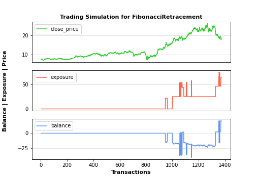
Execute simulation based on trading signals
simulation_data, simulation_statistics, simulation_graph = \
fr_indicator.getTiSimulation(
close_values=df[[‘close’]], max_exposure=None,
short_exposure_factor=1.5)
print(‘\nSimulation Data:\n’, simulation_data)
print(‘\nSimulation Statistics:\n’, simulation_statistics)
Save the Graph for the executed trading signal simulation
simulation_graph.savefig(‘../TTI/simulation_fr.png’)
print(‘\nGraph for the executed trading signal simulation, saved.’)
Technical Indicator value at 2022-06-15: [26.2, 21.6204, 18.7873, 16.4975, 14.2077, 6.795]

Most recent Technical Indicator value: [26.2, 21.6204, 18.7873, 16.4975, 14.2077, 6.795]

Technical Indicator signal: ('hold', 0)
Graph for the calculated fr indicator data, saved.

Simulation Data:
            signal open_trading_action stock_value exposure portfolio_value  \
Date
2017-01-03   hold                none        7.37      0.0             0.0
2017-01-04   hold                none       7.565      0.0             0.0
2017-01-05   hold                none        7.51      0.0             0.0
2017-01-06   hold                none        7.41      0.0             0.0
2017-01-09   hold                none        7.48      0.0             0.0
...           ...                 ...         ...      ...             ...
2022-06-10    buy                long       18.33    64.39           18.33
2022-06-13   hold                none       17.85    64.39           17.85
2022-06-14   hold                none       18.24    64.39           18.24
2022-06-15   hold                none   18.290001    64.39       18.290001
2022-06-16   hold                none       17.67    64.39           17.67

            earnings    balance
Date
2017-01-03       0.0        0.0
2017-01-04       0.0        0.0
2017-01-05       0.0        0.0
2017-01-06       0.0        0.0
2017-01-09       0.0        0.0
...              ...        ...
2022-06-10  3.020002  21.350002
2022-06-13  3.020002  20.870003
2022-06-14  3.020002  21.260002
2022-06-15  3.020002  21.310003
2022-06-16  3.020002  20.690002

[1374 rows x 7 columns]

Simulation Statistics:
 {'number_of_trading_days': 1374, 'number_of_buy_signals': 8, 'number_of_ignored_buy_signals': 0, 'number_of_sell_signals': 10, 'number_of_ignored_sell_signals': 0, 'last_stock_value': 17.67, 'last_exposure': 64.39, 'last_open_long_positions': 2, 'last_open_short_positions': 1, 'last_portfolio_value': 17.67, 'last_earnings': 3.02, 'final_balance': 20.69}

Graph for the executed trading signal simulation, saved.
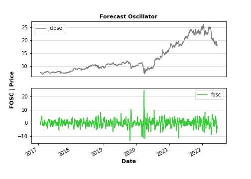
Let’s look at the Forecast Oscillator (FO) that compares actual price with the value returned by the Time Series Forecast study. It is calculated as percentage ratio of the difference between the Close price and previous bar’s Time Series Forecast value to the Close price. The Forecast Oscillator and therefore the time series forecast are based on linear regression. The time series forecast indicator is equal to the sum of two other indicators: the linear regression and the linear regression slope.
from tti.indicators import ForecastOscillator
fo_indicator = ForecastOscillator(input_data=df)
Get indicator’s value for a specific date
print(‘\nTechnical Indicator value at 2022-06-15:’, fo_indicator.getTiValue(‘2022-06-15’))
Get the most recent indicator’s value
print(‘\nMost recent Technical Indicator value:’, fo_indicator.getTiValue())
Get signal from indicator
print(‘\nTechnical Indicator signal:’, fo_indicator.getTiSignal())
Show the Graph for the calculated Technical Indicator
fo_indicator.getTiGraph().show()
Save the Graph for the calculated Technical Indicator
fo_indicator.getTiGraph().savefig(‘../TTI/example_fo.png’)
print(‘\nGraph for the calculated fo indicator data, saved.’)
Execute simulation based on trading signals
simulation_data, simulation_statistics, simulation_graph = \
fo_indicator.getTiSimulation(
close_values=df[[‘close’]], max_exposure=None,
short_exposure_factor=1.5)
print(‘\nSimulation Data:\n’, simulation_data)
print(‘\nSimulation Statistics:\n’, simulation_statistics)
Save the Graph for the executed trading signal simulation
simulation_graph.savefig(‘../TTI/simulation_fo.png’)
print(‘\nGraph for the executed trading signal simulation, saved.’)
Technical Indicator value at 2022-06-15: [-1.9798]

Most recent Technical Indicator value: [-3.9943]

Technical Indicator signal: ('hold', 0)
Graph for the calculated fo indicator data, saved.

Simulation Data:
            signal open_trading_action stock_value    exposure portfolio_value  \
Date
2017-01-03   hold                none        7.37         0.0             0.0
2017-01-04   hold                none       7.565         0.0             0.0
2017-01-05   hold                none        7.51         0.0             0.0
2017-01-06   hold                none        7.41         0.0             0.0
2017-01-09   hold                none        7.48         0.0             0.0
...           ...                 ...         ...         ...             ...
2022-06-10   hold                none       18.33  152.354999          -36.66
2022-06-13   hold                none       17.85  152.354999      -35.700001
2022-06-14   hold                none       18.24  152.354999          -36.48
2022-06-15   hold                none   18.290001  152.354999      -36.580002
2022-06-16   hold                none       17.67  152.354999          -35.34

             earnings    balance
Date
2017-01-03        0.0        0.0
2017-01-04        0.0        0.0
2017-01-05        0.0        0.0
2017-01-06        0.0        0.0
2017-01-09        0.0        0.0
...               ...        ...
2022-06-10  49.379995  12.719995
2022-06-13  49.379995  13.679995
2022-06-14  49.379995  12.899996
2022-06-15  49.379995  12.799994
2022-06-16  49.379995  14.039995

[1374 rows x 7 columns]

Simulation Statistics:
 {'number_of_trading_days': 1374, 'number_of_buy_signals': 153, 'number_of_ignored_buy_signals': 0, 'number_of_sell_signals': 152, 'number_of_ignored_sell_signals': 0, 'last_stock_value': 17.67, 'last_exposure': 152.35, 'last_open_long_positions': 3, 'last_open_short_positions': 5, 'last_portfolio_value': -35.34, 'last_earnings': 49.38, 'final_balance': 14.04}

Graph for the executed trading signal simulation, saved.

Let’s look at the Ichimoku cloud (IMC) trading that attempts to identify a probable direction of price. It helps the trader determine the most suitable time to enter and exit the market by providing you with the trend direction. It gives you reliable support and resistance levels and the strength of these market signals:
from tti.indicators import IchimokuCloud
imc_indicator = IchimokuCloud(input_data=df)
Get indicator’s value for a specific date
print(‘\nTechnical Indicator value at 2022-06-15:’, imc_indicator.getTiValue(‘2022-06-15’))
Get the most recent indicator’s value
print(‘\nMost recent Technical Indicator value:’, imc_indicator.getTiValue())
Get signal from indicator
print(‘\nTechnical Indicator signal:’, imc_indicator.getTiSignal())
Show the Graph for the calculated Technical Indicator
imc_indicator.getTiGraph().show()
Save the Graph for the calculated Technical Indicator
imc_indicator.getTiGraph().savefig(‘../TTI/example_imc.png’)
print(‘\nGraph for the calculated fo indicator data, saved.’)
Execute simulation based on trading signals
simulation_data, simulation_statistics, simulation_graph = \
imc_indicator.getTiSimulation(
close_values=df[[‘close’]], max_exposure=None,
short_exposure_factor=1.5)
print(‘\nSimulation Data:\n’, simulation_data)
print(‘\nSimulation Statistics:\n’, simulation_statistics)
Save the Graph for the executed trading signal simulation
simulation_graph.savefig(‘../TTI/simulation_imc.png’)
print(‘\nGraph for the executed trading signal simulation, saved.’)
Technical Indicator value at 2022-06-15: [18.7, 18.94, 21.335, 22.46]

Most recent Technical Indicator value: [18.62, 18.685, 21.1425, 22.365]

Technical Indicator signal: ('hold', 0)

Graph for the calculated fo indicator data, saved.

Simulation Data:
            signal open_trading_action stock_value exposure portfolio_value  \
Date
2017-01-03   hold                none        7.37      0.0             0.0
2017-01-04   hold                none       7.565      0.0             0.0
2017-01-05   hold                none        7.51      0.0             0.0
2017-01-06   hold                none        7.41      0.0             0.0
2017-01-09   hold                none        7.48      0.0             0.0
...           ...                 ...         ...      ...             ...
2022-06-10   hold                none       18.33      0.0             0.0
2022-06-13   hold                none       17.85      0.0             0.0
2022-06-14   hold                none       18.24      0.0             0.0
2022-06-15   hold                none   18.290001      0.0             0.0
2022-06-16   hold                none       17.67      0.0             0.0

           earnings balance
Date
2017-01-03      0.0     0.0
2017-01-04      0.0     0.0
2017-01-05      0.0     0.0
2017-01-06      0.0     0.0
2017-01-09      0.0     0.0
...             ...     ...
2022-06-10     0.79    0.79
2022-06-13     0.79    0.79
2022-06-14     0.79    0.79
2022-06-15     0.79    0.79
2022-06-16     0.79    0.79

[1374 rows x 7 columns]

Simulation Statistics:
 {'number_of_trading_days': 1374, 'number_of_buy_signals': 5, 'number_of_ignored_buy_signals': 0, 'number_of_sell_signals': 1, 'number_of_ignored_sell_signals': 0, 'last_stock_value': 17.67, 'last_exposure': 0.0, 'last_open_long_positions': 0, 'last_open_short_positions': 0, 'last_portfolio_value': 0.0, 'last_earnings': 0.79, 'final_balance': 0.79}

Graph for the executed trading signal simulation, saved.

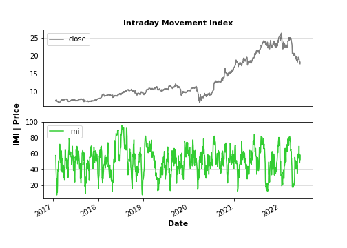
Let’s look at the Intraday Momentum Index (IMI) – a technical indicator that combines aspects of candlestick analysis with the relative strength index (RSI) in order to generate overbought or oversold signals. The intraday indicator was developed by market technician Tushar Chande to aid investors with their trading decisions.
from tti.indicators import IntradayMovementIndex
idmi_indicator = IntradayMovementIndex(input_data=df)
Get indicator’s value for a specific date
print(‘\nTechnical Indicator value at 2022-06-15:’, idmi_indicator.getTiValue(‘2022-06-15’))
Get the most recent indicator’s value
print(‘\nMost recent Technical Indicator value:’, idmi_indicator.getTiValue())
Get signal from indicator
print(‘\nTechnical Indicator signal:’, idmi_indicator.getTiSignal())
Show the Graph for the calculated Technical Indicator
idmi_indicator.getTiGraph().show()
Save the Graph for the calculated Technical Indicator
idmi_indicator.getTiGraph().savefig(‘../TTI/example_idmi.png’)
print(‘\nGraph for the calculated fo indicator data, saved.’)
Execute simulation based on trading signals
simulation_data, simulation_statistics, simulation_graph = \
idmi_indicator.getTiSimulation(
close_values=df[[‘close’]], max_exposure=None,
short_exposure_factor=1.5)
print(‘\nSimulation Data:\n’, simulation_data)
print(‘\nSimulation Statistics:\n’, simulation_statistics)
Save the Graph for the executed trading signal simulation
simulation_graph.savefig(‘../TTI/simulation_idmi.png’)
print(‘\nGraph for the executed trading signal simulation, saved.’)
Technical Indicator value at 2022-06-15: [58.6614]

Most recent Technical Indicator value: [52.5]

Technical Indicator signal: ('hold', 0)
Graph for the calculated fo indicator data, saved.

Simulation Data:
            signal open_trading_action stock_value   exposure portfolio_value  \
Date
2017-01-03   hold                none        7.37        0.0             0.0
2017-01-04   hold                none       7.565        0.0             0.0
2017-01-05   hold                none        7.51        0.0             0.0
2017-01-06   hold                none        7.41        0.0             0.0
2017-01-09   hold                none        7.48        0.0             0.0
...           ...                 ...         ...        ...             ...
2022-06-10   hold                none       18.33  61.885001          -18.33
2022-06-13   hold                none       17.85  61.885001          -17.85
2022-06-14   hold                none       18.24  61.885001          -18.24
2022-06-15   hold                none   18.290001  61.885001      -18.290001
2022-06-16   hold                none       17.67  61.885001          -17.67

            earnings   balance
Date
2017-01-03       0.0       0.0
2017-01-04       0.0       0.0
2017-01-05       0.0       0.0
2017-01-06       0.0       0.0
2017-01-09       0.0       0.0
...              ...       ...
2022-06-10  9.934999 -8.395001
2022-06-13  9.934999 -7.915001
2022-06-14  9.934999 -8.305001
2022-06-15  9.934999 -8.355002
2022-06-16  9.934999 -7.735001

[1374 rows x 7 columns]

Simulation Statistics:
 {'number_of_trading_days': 1374, 'number_of_buy_signals': 37, 'number_of_ignored_buy_signals': 0, 'number_of_sell_signals': 33, 'number_of_ignored_sell_signals': 0, 'last_stock_value': 17.67, 'last_exposure': 61.89, 'last_open_long_positions': 1, 'last_open_short_positions': 2, 'last_portfolio_value': -17.67, 'last_earnings': 9.93, 'final_balance': -7.74}

Graph for the executed trading signal simulation, saved.

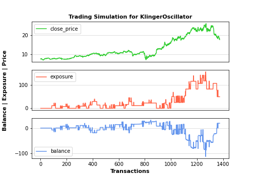
Let’s look at the Klinger oscillator (KO) – a financial tool that was designed by Stephen Klinger in 1977 to predict long-term trends in money flow while also detecting short-term fluctuations. In addition, it predicts price reversals in a financial market by extensively comparing volume to price:
from tti.indicators import KlingerOscillator
klo_indicator = KlingerOscillator(input_data=df)
Get indicator’s value for a specific date
print(‘\nTechnical Indicator value at 2022-06-15:’, klo_indicator.getTiValue(‘2022-06-15’))
Get the most recent indicator’s value
print(‘\nMost recent Technical Indicator value:’, klo_indicator.getTiValue())
Get signal from indicator
print(‘\nTechnical Indicator signal:’, klo_indicator.getTiSignal())
Show the Graph for the calculated Technical Indicator
klo_indicator.getTiGraph().show()
Save the Graph for the calculated Technical Indicator
klo_indicator.getTiGraph().savefig(‘../TTI/example_klo.png’)
print(‘\nGraph for the calculated fo indicator data, saved.’)
Execute simulation based on trading signals
simulation_data, simulation_statistics, simulation_graph = \
klo_indicator.getTiSimulation(
close_values=df[[‘close’]], max_exposure=None,
short_exposure_factor=1.5)
print(‘\nSimulation Data:\n’, simulation_data)
print(‘\nSimulation Statistics:\n’, simulation_statistics)
Save the Graph for the executed trading signal simulation
simulation_graph.savefig(‘../TTI/simulation_klo.png’)
print(‘\nGraph for the executed trading signal simulation, saved.’)
Technical Indicator value at 2022-06-15: [12512248.6986]

Most recent Technical Indicator value: [7423476.0864]

Technical Indicator signal: ('hold', 0)

Graph for the calculated fo indicator data, saved.

Simulation Data:
            signal open_trading_action stock_value   exposure portfolio_value  \
Date
2017-01-03   hold                none        7.37        0.0             0.0
2017-01-04   hold                none       7.565        0.0             0.0
2017-01-05   hold                none        7.51        0.0             0.0
2017-01-06   hold                none        7.41        0.0             0.0
2017-01-09   hold                none        7.48        0.0             0.0
...           ...                 ...         ...        ...             ...
2022-06-10   hold                none       18.33  49.249999             0.0
2022-06-13   hold                none       17.85  49.249999             0.0
2022-06-14   hold                none       18.24  49.249999             0.0
2022-06-15   hold                none   18.290001  49.249999             0.0
2022-06-16   hold                none       17.67  49.249999             0.0

             earnings    balance
Date
2017-01-03        0.0        0.0
2017-01-04        0.0        0.0
2017-01-05        0.0        0.0
2017-01-06        0.0        0.0
2017-01-09        0.0        0.0
...               ...        ...
2022-06-10  18.905005  18.905005
2022-06-13  18.905005  18.905005
2022-06-14  18.905005  18.905005
2022-06-15  18.905005  18.905005
2022-06-16  18.905005  18.905005

[1374 rows x 7 columns]

Simulation Statistics:
 {'number_of_trading_days': 1374, 'number_of_buy_signals': 59, 'number_of_ignored_buy_signals': 0, 'number_of_sell_signals': 60, 'number_of_ignored_sell_signals': 0, 'last_stock_value': 17.67, 'last_exposure': 49.25, 'last_open_long_positions': 1, 'last_open_short_positions': 1, 'last_portfolio_value': 0.0, 'last_earnings': 18.91, 'final_balance': 18.91}

Graph for the executed trading signal simulation, saved.
Let’s look at the Linear Regression (LREG) Indicator that plots the ending value of a Linear Regression Line for a specified number of bars; showing, statistically, where the price is expected to be. For example, a 20 period Linear Regression Indicator will equal the ending value of a Linear Regression line that covers 20 bars.
from tti.indicators import LinearRegressionIndicator
lreg_indicator = LinearRegressionIndicator(input_data=df)
Get indicator’s value for a specific date
print(‘\nTechnical Indicator value at 2022-06-15:’, lreg_indicator.getTiValue(‘2022-06-15’))
Get the most recent indicator’s value
print(‘\nMost recent Technical Indicator value:’, lreg_indicator.getTiValue())
Get signal from indicator
print(‘\nTechnical Indicator signal:’, lreg_indicator.getTiSignal())
Show the Graph for the calculated Technical Indicator
lreg_indicator.getTiGraph().show()
Save the Graph for the calculated Technical Indicator
lreg_indicator.getTiGraph().savefig(‘../TTI/example_lreg.png’)
print(‘\nGraph for the calculated fo indicator data, saved.’)
Execute simulation based on trading signals
simulation_data, simulation_statistics, simulation_graph = \
lreg_indicator.getTiSimulation(
close_values=df[[‘close’]], max_exposure=None,
short_exposure_factor=1.5)
print(‘\nSimulation Data:\n’, simulation_data)
print(‘\nSimulation Statistics:\n’, simulation_statistics)
Save the Graph for the executed trading signal simulation
simulation_graph.savefig(‘../TTI/simulation_lreg.png’)
print(‘\nGraph for the executed trading signal simulation, saved.’)
Technical Indicator value at 2022-06-15: [18.438]

Most recent Technical Indicator value: [18.0806]

Technical Indicator signal: ('hold', 0)

Graph for the calculated fo indicator data, saved.

Simulation Data:
            signal open_trading_action stock_value exposure portfolio_value  \
Date
2017-01-03   hold                none        7.37      0.0             0.0
2017-01-04   hold                none       7.565      0.0             0.0
2017-01-05   hold                none        7.51      0.0             0.0
2017-01-06   hold                none        7.41      0.0             0.0
2017-01-09   hold                none        7.48      0.0             0.0
...           ...                 ...         ...      ...             ...
2022-06-10   hold                none       18.33  117.055          -36.66
2022-06-13   hold                none       17.85  117.055      -35.700001
2022-06-14   hold                none       18.24  117.055          -36.48
2022-06-15   hold                none   18.290001  117.055      -36.580002
2022-06-16   hold                none       17.67  117.055          -35.34

             earnings    balance
Date
2017-01-03        0.0        0.0
2017-01-04        0.0        0.0
2017-01-05        0.0        0.0
2017-01-06        0.0        0.0
2017-01-09        0.0        0.0
...               ...        ...
2022-06-10  55.309997  18.649997
2022-06-13  55.309997  19.609996
2022-06-14  55.309997  18.829997
2022-06-15  55.309997  18.729995
2022-06-16  55.309997  19.969996

[1374 rows x 7 columns]

Simulation Statistics:
 {'number_of_trading_days': 1374, 'number_of_buy_signals': 169, 'number_of_ignored_buy_signals': 0, 'number_of_sell_signals': 169, 'number_of_ignored_sell_signals': 0, 'last_stock_value': 17.67, 'last_exposure': 117.05, 'last_open_long_positions': 2, 'last_open_short_positions': 4, 'last_portfolio_value': -35.34, 'last_earnings': 55.31, 'final_balance': 19.97}

Graph for the executed trading signal simulation, saved.

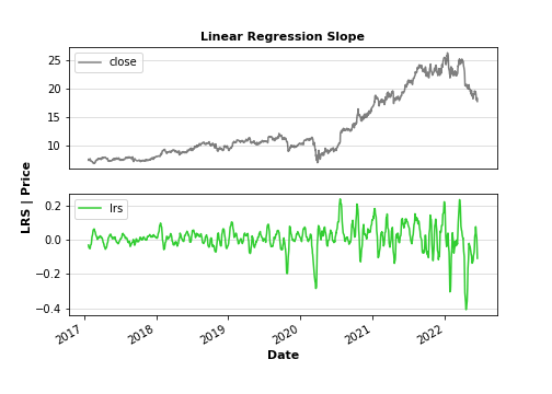
It is useful to consider the Linear Regression Slope Indicator – a centered oscillator type of indicator which is similar to momentum indicators. The momentum is positive when the Slope is above 0 and negative when it is below 0. We can use this indicator to measure the strength or weakness and direction of the momentum.
from tti.indicators import LinearRegressionSlope
slop_indicator = LinearRegressionSlope(input_data=df)
Get indicator’s value for a specific date
print(‘\nTechnical Indicator value at 2022-06-15:’, slop_indicator.getTiValue(‘2022-06-15’))
Get the most recent indicator’s value
print(‘\nMost recent Technical Indicator value:’, slop_indicator.getTiValue())
Get signal from indicator
print(‘\nTechnical Indicator signal:’, slop_indicator.getTiSignal())
Show the Graph for the calculated Technical Indicator
slop_indicator.getTiGraph().show()
Save the Graph for the calculated Technical Indicator
slop_indicator.getTiGraph().savefig(‘../TTI/example_slop.png’)
print(‘\nGraph for the calculated fo indicator data, saved.’)
Execute simulation based on trading signals
simulation_data, simulation_statistics, simulation_graph = \
slop_indicator.getTiSimulation(
close_values=df[[‘close’]], max_exposure=None,
short_exposure_factor=1.5)
print(‘\nSimulation Data:\n’, simulation_data)
print(‘\nSimulation Statistics:\n’, simulation_statistics)
Save the Graph for the executed trading signal simulation
simulation_graph.savefig(‘../TTI/simulation_slop.png’)
print(‘\nGraph for the executed trading signal simulation, saved.’)
Technical Indicator value at 2022-06-15: [-0.0622]

Most recent Technical Indicator value: [-0.1086]

Technical Indicator signal: ('hold', 0)
Graph for the calculated fo indicator data, saved.

Simulation Data:
            signal open_trading_action stock_value   exposure portfolio_value  \
Date
2017-01-03   hold                none        7.37        0.0             0.0
2017-01-04   hold                none       7.565        0.0             0.0
2017-01-05   hold                none        7.51        0.0             0.0
2017-01-06   hold                none        7.41        0.0             0.0
2017-01-09   hold                none        7.48        0.0             0.0
...           ...                 ...         ...        ...             ...
2022-06-10   hold                none       18.33  50.594999          -18.33
2022-06-13   hold                none       17.85  50.594999          -17.85
2022-06-14    buy                long       18.24  68.834999             0.0
2022-06-15   hold                none   18.290001  50.594999      -18.290001
2022-06-16   hold                none       17.67  50.594999          -17.67

             earnings    balance
Date
2017-01-03        0.0        0.0
2017-01-04        0.0        0.0
2017-01-05        0.0        0.0
2017-01-06        0.0        0.0
2017-01-09        0.0        0.0
...               ...        ...
2022-06-10  16.434991  -1.895009
2022-06-13  16.434991  -1.415009
2022-06-14  16.434991  16.434991
2022-06-15  16.484993  -1.805008
2022-06-16  16.484993  -1.185008

[1374 rows x 7 columns]

Simulation Statistics:
 {'number_of_trading_days': 1374, 'number_of_buy_signals': 52, 'number_of_ignored_buy_signals': 0, 'number_of_sell_signals': 52, 'number_of_ignored_sell_signals': 0, 'last_stock_value': 17.67, 'last_exposure': 50.59, 'last_open_long_positions': 1, 'last_open_short_positions': 2, 'last_portfolio_value': -17.67, 'last_earnings': 16.48, 'final_balance': -1.19}

Graph for the executed trading signal simulation, saved.

Let’s look at the market facilitation index (MFI) – an indicator that measures the strength or weakness behind movements of the price of an asset.
The MFI indicator can help you decide when a price trend is strong enough to justify trading it, when a new trend may be about to start and when to avoid entering trades altogether.
It does this by looking at changes in the size of price moves and whether the trading volume is rising or falling.
from tti.indicators import MarketFacilitationIndex
mfi_indicator = MarketFacilitationIndex(input_data=df)
Get indicator’s value for a specific date
print(‘\nTechnical Indicator value at 2022-06-15:’, mfi_indicator.getTiValue(‘2022-06-15’))
Get the most recent indicator’s value
print(‘\nMost recent Technical Indicator value:’, mfi_indicator.getTiValue())
Get signal from indicator
print(‘\nTechnical Indicator signal:’, mfi_indicator.getTiSignal())
Show the Graph for the calculated Technical Indicator
mfi_indicator.getTiGraph().show()
Save the Graph for the calculated Technical Indicator
mfi_indicator.getTiGraph().savefig(‘../TTI/example_mfi.png’)
print(‘\nGraph for the calculated fo indicator data, saved.’)
Execute simulation based on trading signals
simulation_data, simulation_statistics, simulation_graph = \
mfi_indicator.getTiSimulation(
close_values=df[[‘close’]], max_exposure=None,
short_exposure_factor=1.5)
print(‘\nSimulation Data:\n’, simulation_data)
print(‘\nSimulation Statistics:\n’, simulation_statistics)
Save the Graph for the executed trading signal simulation
simulation_graph.savefig(‘../TTI/simulation_mfi.png’)
print(‘\nGraph for the executed trading signal simulation, saved.’)
Technical Indicator value at 2022-06-15: [2.6e-08]

Most recent Technical Indicator value: [3.27e-08]

Technical Indicator signal: ('sell', 1)

Graph for the calculated fo indicator data, saved.

Simulation Data:
            signal open_trading_action stock_value    exposure portfolio_value  \
Date
2017-01-03   hold                none        7.37         0.0             0.0
2017-01-04   sell               short       7.565     11.3475          -7.565
2017-01-05    buy                long        7.51        7.51            7.51
2017-01-06   sell               short        7.41      18.625             0.0
2017-01-09   sell               short        7.48      29.845           -7.48
...           ...                 ...         ...         ...             ...
2022-06-10    buy                long       18.33  892.622498     -274.949999
2022-06-13    buy                long       17.85  910.472498     -249.900005
2022-06-14    buy                long       18.24  910.862498     -255.359997
2022-06-15    buy                long   18.290001  910.912499     -256.060013
2022-06-16   sell               short       17.67  910.657499     -247.380001

              earnings    balance
Date
2017-01-03         0.0        0.0
2017-01-04         0.0     -7.565
2017-01-05       0.055      7.565
2017-01-06       0.055      0.055
2017-01-09       0.055     -7.425
...                ...        ...
2022-06-10  209.124999    -65.825
2022-06-13  209.124999 -40.775007
2022-06-14  209.514998 -45.844999
2022-06-15  209.564999 -46.495014
2022-06-16  209.734999 -37.645002

[1374 rows x 7 columns]

Simulation Statistics:
 {'number_of_trading_days': 1374, 'number_of_buy_signals': 686, 'number_of_ignored_buy_signals': 0, 'number_of_sell_signals': 683, 'number_of_ignored_sell_signals': 0, 'last_stock_value': 17.67, 'last_exposure': 910.66, 'last_open_long_positions': 16, 'last_open_short_positions': 30, 'last_portfolio_value': -247.38, 'last_earnings': 209.73, 'final_balance': -37.65}

Graph for the executed trading signal simulation, saved.

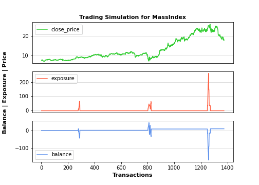
Let’s look at the mass index (MI) – an indicator, developed by Donald Dorsey, used in technical analysis to predict trend reversals. It is based on the notion that there is a tendency for reversal when the price range widens, and therefore compares previous trading ranges (highs minus lows).
from tti.indicators import MassIndex
mind_indicator = MassIndex(input_data=df)
Get indicator’s value for a specific date
print(‘\nTechnical Indicator value at 2022-06-15:’, mind_indicator.getTiValue(‘2022-06-15’))
Get the most recent indicator’s value
print(‘\nMost recent Technical Indicator value:’, mind_indicator.getTiValue())
Get signal from indicator
print(‘\nTechnical Indicator signal:’, mind_indicator.getTiSignal())
Show the Graph for the calculated Technical Indicator
mind_indicator.getTiGraph().show()
Save the Graph for the calculated Technical Indicator
mind_indicator.getTiGraph().savefig(‘../TTI/example_mind.png’)
print(‘\nGraph for the calculated fo indicator data, saved.’)
Execute simulation based on trading signals
simulation_data, simulation_statistics, simulation_graph = \
mind_indicator.getTiSimulation(
close_values=df[[‘close’]], max_exposure=None,
short_exposure_factor=1.5)
print(‘\nSimulation Data:\n’, simulation_data)
print(‘\nSimulation Statistics:\n’, simulation_statistics)
Save the Graph for the executed trading signal simulation
simulation_graph.savefig(‘../TTI/simulation_mind.png’)
print(‘\nGraph for the executed trading signal simulation, saved.’)
Technical Indicator value at 2022-06-15: [24.0192]

Most recent Technical Indicator value: [23.9409]

Technical Indicator signal: ('hold', 0)

Graph for the calculated fo indicator data, saved.

Simulation Data:
            signal open_trading_action stock_value exposure portfolio_value  \
Date
2017-01-03   hold                none        7.37      0.0             0.0
2017-01-04   hold                none       7.565      0.0             0.0
2017-01-05   hold                none        7.51      0.0             0.0
2017-01-06   hold                none        7.41      0.0             0.0
2017-01-09   hold                none        7.48      0.0             0.0
...           ...                 ...         ...      ...             ...
2022-06-10   hold                none       18.33      0.0             0.0
2022-06-13   hold                none       17.85      0.0             0.0
2022-06-14   hold                none       18.24      0.0             0.0
2022-06-15   hold                none   18.290001      0.0             0.0
2022-06-16   hold                none       17.67      0.0             0.0

           earnings balance
Date
2017-01-03      0.0     0.0
2017-01-04      0.0     0.0
2017-01-05      0.0     0.0
2017-01-06      0.0     0.0
2017-01-09      0.0     0.0
...             ...     ...
2022-06-10    9.335   9.335
2022-06-13    9.335   9.335
2022-06-14    9.335   9.335
2022-06-15    9.335   9.335
2022-06-16    9.335   9.335

[1374 rows x 7 columns]

Simulation Statistics:
 {'number_of_trading_days': 1374, 'number_of_buy_signals': 16, 'number_of_ignored_buy_signals': 0, 'number_of_sell_signals': 27, 'number_of_ignored_sell_signals': 0, 'last_stock_value': 17.67, 'last_exposure': 0.0, 'last_open_long_positions': 0, 'last_open_short_positions': 0, 'last_portfolio_value': 0.0, 'last_earnings': 9.34, 'final_balance': 9.34}
Graph for the executed trading signal simulation, saved.
Let’s look at the Median Price (MP) indicator. MP is simply the midpoint of each day’s price. The Typical Price and Weighted Close are similar indicators. The MP indicator provides a simple, single-line chart of the day’s “average price.” This average price is useful when you want a simpler view of prices.
from tti.indicators import MedianPrice
medp_indicator = MedianPrice(input_data=df)
Get indicator’s value for a specific date
print(‘\nTechnical Indicator value at 2022-06-15:’, medp_indicator.getTiValue(‘2022-06-15’))
Get the most recent indicator’s value
print(‘\nMost recent Technical Indicator value:’, medp_indicator.getTiValue())
Get signal from indicator
print(‘\nTechnical Indicator signal:’, medp_indicator.getTiSignal())
Show the Graph for the calculated Technical Indicator
medp_indicator.getTiGraph().show()
Save the Graph for the calculated Technical Indicator
medp_indicator.getTiGraph().savefig(‘C:/Users/adrou/OneDrive/Documents/TTI/example_medp.png’)
print(‘\nGraph for the calculated fo indicator data, saved.’)
Execute simulation based on trading signals
simulation_data, simulation_statistics, simulation_graph = \
medp_indicator.getTiSimulation(
close_values=df[[‘close’]], max_exposure=None,
short_exposure_factor=1.5)
print(‘\nSimulation Data:\n’, simulation_data)
print(‘\nSimulation Statistics:\n’, simulation_statistics)
Save the Graph for the executed trading signal simulation
simulation_graph.savefig(‘../TTI/simulation_medp.png’)
print(‘\nGraph for the executed trading signal simulation, saved.’)
Technical Indicator value at 2022-06-15: [18.115]

Most recent Technical Indicator value: [17.695]

Technical Indicator signal: ('hold', 0)
Graph for the calculated fo indicator data, saved.

Simulation Data:
            signal open_trading_action stock_value    exposure portfolio_value  \
Date
2017-01-03   hold                none        7.37         0.0             0.0
2017-01-04   hold                none       7.565         0.0             0.0
2017-01-05   hold                none        7.51         0.0             0.0
2017-01-06   hold                none        7.41         0.0             0.0
2017-01-09   hold                none        7.48         0.0             0.0
...           ...                 ...         ...         ...             ...
2022-06-10   hold                none       18.33  115.664999          -36.66
2022-06-13   hold                none       17.85  115.664999      -35.700001
2022-06-14   hold                none       18.24  115.664999          -36.48
2022-06-15   hold                none   18.290001  115.664999      -36.580002
2022-06-16   hold                none       17.67  115.664999          -35.34

             earnings   balance
Date
2017-01-03        0.0       0.0
2017-01-04        0.0       0.0
2017-01-05        0.0       0.0
2017-01-06        0.0       0.0
2017-01-09        0.0       0.0
...               ...       ...
2022-06-10  29.144997 -7.515003
2022-06-13  29.144997 -6.555004
2022-06-14  29.144997 -7.335003
2022-06-15  29.144997 -7.435005
2022-06-16  29.144997 -6.195004

[1374 rows x 7 columns]

Simulation Statistics:
 {'number_of_trading_days': 1374, 'number_of_buy_signals': 92, 'number_of_ignored_buy_signals': 0, 'number_of_sell_signals': 92, 'number_of_ignored_sell_signals': 0, 'last_stock_value': 17.67, 'last_exposure': 115.66, 'last_open_long_positions': 2, 'last_open_short_positions': 4, 'last_portfolio_value': -35.34, 'last_earnings': 29.14, 'final_balance': -6.2}

Graph for the executed trading signal simulation, saved.

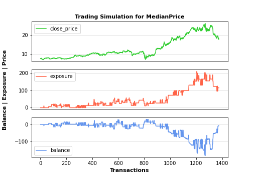
Let’s look at the momentum indicator (oscillator) – a technical indicator which shows the trend direction and measures the pace of the price fluctuation by comparing current and past values. It is one of the leading indicators that measure the rate of change of securities. A momentum indicator is generally used in unison with other indicators.
from tti.indicators import Momentum
mom_indicator = Momentum(input_data=df)
Get indicator’s value for a specific date
print(‘\nTechnical Indicator value at 2022-06-15:’, mom_indicator.getTiValue(‘2022-06-15’))
Get the most recent indicator’s value
print(‘\nMost recent Technical Indicator value:’, mom_indicator.getTiValue())
Get signal from indicator
print(‘\nTechnical Indicator signal:’, mom_indicator.getTiSignal())
Show the Graph for the calculated Technical Indicator
mom_indicator.getTiGraph().show()
Save the Graph for the calculated Technical Indicator
mom_indicator.getTiGraph().savefig(‘../TTI/example_mom.png’)
print(‘\nGraph for the calculated fo indicator data, saved.’)
Execute simulation based on trading signals
simulation_data, simulation_statistics, simulation_graph = \
mom_indicator.getTiSimulation(
close_values=df[[‘close’]], max_exposure=None,
short_exposure_factor=1.5)
print(‘\nSimulation Data:\n’, simulation_data)
print(‘\nSimulation Statistics:\n’, simulation_statistics)
Save the Graph for the executed trading signal simulation
simulation_graph.savefig(‘../TTI/simulation_mom.png’)
print(‘\nGraph for the executed trading signal simulation, saved.’)
Technical Indicator value at 2022-06-15: [96.2632]

Most recent Technical Indicator value: [93.6903]

Technical Indicator signal: ('hold', 0)

Graph for the calculated fo indicator data, saved.

Simulation Data:
            signal open_trading_action stock_value exposure portfolio_value  \
Date
2017-01-03   hold                none        7.37      0.0             0.0
2017-01-04   hold                none       7.565      0.0             0.0
2017-01-05   hold                none        7.51      0.0             0.0
2017-01-06   hold                none        7.41      0.0             0.0
2017-01-09   hold                none        7.48      0.0             0.0
...           ...                 ...         ...      ...             ...
2022-06-10   hold                none       18.33   77.465             0.0
2022-06-13   hold                none       17.85   77.465             0.0
2022-06-14   hold                none       18.24   77.465             0.0
2022-06-15   hold                none   18.290001   77.465             0.0
2022-06-16   hold                none       17.67   77.465             0.0

             earnings    balance
Date
2017-01-03        0.0        0.0
2017-01-04        0.0        0.0
2017-01-05        0.0        0.0
2017-01-06        0.0        0.0
2017-01-09        0.0        0.0
...               ...        ...
2022-06-10  43.729992  43.729992
2022-06-13  43.729992  43.729992
2022-06-14  43.729992  43.729992
2022-06-15  43.729992  43.729992
2022-06-16  43.729992  43.729992

[1374 rows x 7 columns]

Simulation Statistics:
 {'number_of_trading_days': 1374, 'number_of_buy_signals': 140, 'number_of_ignored_buy_signals': 0, 'number_of_sell_signals': 139, 'number_of_ignored_sell_signals': 0, 'last_stock_value': 17.67, 'last_exposure': 77.46, 'last_open_long_positions': 2, 'last_open_short_positions': 2, 'last_portfolio_value': 0.0, 'last_earnings': 43.73, 'final_balance': 43.73}

Graph for the executed trading signal simulation, saved.

Let’s look at the moving average (MVA) – a technical indicator that investors and traders use to determine the trend direction of securities. It is calculated by adding up all the data points during a specific period and dividing the sum by the number of time periods. Moving averages help technical traders to generate trading signals.
from tti.indicators import MovingAverage
mva_indicator = MovingAverage(input_data=df,period=50)
Get indicator’s value for a specific date
print(‘\nTechnical Indicator value at 2022-06-15:’, mva_indicator.getTiValue(‘2022-06-15’))
Get the most recent indicator’s value
print(‘\nMost recent Technical Indicator value:’, mva_indicator.getTiValue())
Get signal from indicator
print(‘\nTechnical Indicator signal:’, mva_indicator.getTiSignal())
Show the Graph for the calculated Technical Indicator
mva_indicator.getTiGraph().show()
Save the Graph for the calculated Technical Indicator
mva_indicator.getTiGraph().savefig(‘../TTI/example_mva.png’)
print(‘\nGraph for the calculated fo indicator data, saved.’)
Execute simulation based on trading signals
simulation_data, simulation_statistics, simulation_graph = \
mva_indicator.getTiSimulation(
close_values=df[[‘close’]], max_exposure=None,
short_exposure_factor=1.5)
print(‘\nSimulation Data:\n’, simulation_data)
print(‘\nSimulation Statistics:\n’, simulation_statistics)
Save the Graph for the executed trading signal simulation
simulation_graph.savefig(‘../TTI/simulation_mva.png’)
print(‘\nGraph for the executed trading signal simulation, saved.’)
Technical Indicator value at 2022-06-15: [19.9928]

Most recent Technical Indicator value: [19.8586]

Technical Indicator signal: ('hold', 0)
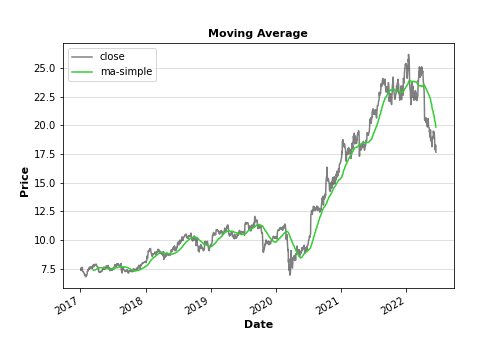
Graph for the calculated fo indicator data, saved.

Simulation Data:
            signal open_trading_action stock_value exposure portfolio_value  \
Date
2017-01-03   hold                none        7.37      0.0             0.0
2017-01-04   hold                none       7.565      0.0             0.0
2017-01-05   hold                none        7.51      0.0             0.0
2017-01-06   hold                none        7.41      0.0             0.0
2017-01-09   hold                none        7.48      0.0             0.0
...           ...                 ...         ...      ...             ...
2022-06-10   hold                none       18.33    272.4      201.629999
2022-06-13   hold                none       17.85    272.4      196.350004
2022-06-14   hold                none       18.24    272.4      200.639997
2022-06-15   hold                none   18.290001    272.4       201.19001
2022-06-16   hold                none       17.67    272.4      194.370001

              earnings     balance
Date
2017-01-03         0.0         0.0
2017-01-04         0.0         0.0
2017-01-05         0.0         0.0
2017-01-06         0.0         0.0
2017-01-09         0.0         0.0
...                ...         ...
2022-06-10  129.670009  331.300008
2022-06-13  129.670009  326.020013
2022-06-14  129.670009  330.310007
2022-06-15  129.670009  330.860019
2022-06-16  129.670009   324.04001

[1374 rows x 7 columns]

Simulation Statistics:
 {'number_of_trading_days': 1374, 'number_of_buy_signals': 863, 'number_of_ignored_buy_signals': 0, 'number_of_sell_signals': 0, 'number_of_ignored_sell_signals': 0, 'last_stock_value': 17.67, 'last_exposure': 272.4, 'last_open_long_positions': 11, 'last_open_short_positions': 0, 'last_portfolio_value': 194.37, 'last_earnings': 129.67, 'final_balance': 324.04}

Graph for the executed trading signal simulation, saved.
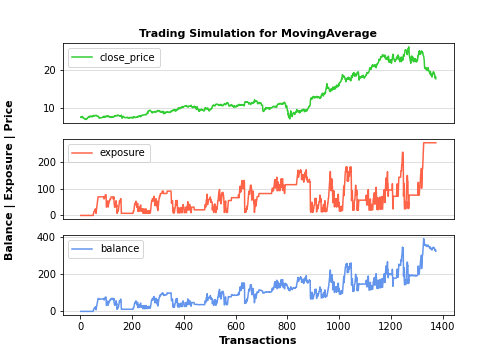
Let’s look at the popular Moving Average Convergence Divergence (MACD) – a trend-following momentum indicator that shows the relationship between two moving averages of a security’s price:
- Traders use the MACD to identify when bullish or bearish momentum is high in order to identify entry and exit points for trades.
- MACD is used by technical traders in stocks, bonds, commodities, and FX markets.
from tti.indicators import MovingAverageConvergenceDivergence
mvacd_indicator = MovingAverageConvergenceDivergence(input_data=df)
Get indicator’s value for a specific date
print(‘\nTechnical Indicator value at 2022-06-15:’, mvacd_indicator.getTiValue(‘2022-06-15’))
Get the most recent indicator’s value
print(‘\nMost recent Technical Indicator value:’, mvacd_indicator.getTiValue())
Get signal from indicator
print(‘\nTechnical Indicator signal:’, mvacd_indicator.getTiSignal())
Show the Graph for the calculated Technical Indicator
mvacd_indicator.getTiGraph().show()
Save the Graph for the calculated Technical Indicator
mvacd_indicator.getTiGraph().savefig(‘C:/Users/adrou/OneDrive/Documents/TTI/example_mvacd.png’)
print(‘\nGraph for the calculated fo indicator data, saved.’)
Execute simulation based on trading signals
simulation_data, simulation_statistics, simulation_graph = \
mvacd_indicator.getTiSimulation(
close_values=df[[‘close’]], max_exposure=None,
short_exposure_factor=1.5)
print(‘\nSimulation Data:\n’, simulation_data)
print(‘\nSimulation Statistics:\n’, simulation_statistics)
Save the Graph for the executed trading signal simulation
simulation_graph.savefig(../TTI/simulation_mvacd.png’)
print(‘\nGraph for the executed trading signal simulation, saved.’)
Technical Indicator value at 2022-06-15: [-0.4465, -0.4459]

Most recent Technical Indicator value: [-0.4928, -0.4553]

Technical Indicator signal: ('hold', 0)

Graph for the calculated fo indicator data, saved.

Simulation Data:
            signal open_trading_action stock_value    exposure portfolio_value  \
Date
2017-01-03   hold                none        7.37         0.0             0.0
2017-01-04   hold                none       7.565         0.0             0.0
2017-01-05   hold                none        7.51         0.0             0.0
2017-01-06   hold                none        7.41         0.0             0.0
2017-01-09   hold                none        7.48         0.0             0.0
...           ...                 ...         ...         ...             ...
2022-06-10   hold                none       18.33      217.35     -146.639999
2022-06-13   hold                none       17.85  190.140001     -124.950003
2022-06-14   hold                none       18.24  190.140001     -127.679998
2022-06-15   sell               short   18.290001  217.575003     -146.320007
2022-06-16   hold                none       17.67  163.380001         -106.02

             earnings     balance
Date
2017-01-03        0.0         0.0
2017-01-04        0.0         0.0
2017-01-05        0.0         0.0
2017-01-06        0.0         0.0
2017-01-09        0.0         0.0
...               ...         ...
2022-06-10  26.075003 -120.564996
2022-06-13  26.365002  -98.585001
2022-06-14  26.365002 -101.314996
2022-06-15  26.365002 -119.955005
2022-06-16  27.155003  -78.864997

[1374 rows x 7 columns]

Simulation Statistics:
 {'number_of_trading_days': 1374, 'number_of_buy_signals': 72, 'number_of_ignored_buy_signals': 0, 'number_of_sell_signals': 74, 'number_of_ignored_sell_signals': 0, 'last_stock_value': 17.67, 'last_exposure': 163.38, 'last_open_long_positions': 1, 'last_open_short_positions': 7, 'last_portfolio_value': -106.02, 'last_earnings': 27.16, 'final_balance': -78.86}

Graph for the executed trading signal simulation, saved.
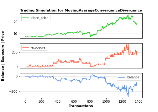
Let’s look at the Negative Volume Index (NVI) – a cumulative indicator, developed by Paul Dysart in the 1930s, that uses the change in volume to decide when the smart money is active. The NVI assumes that smart money will produce moves in price that require less volume than the rest of the investment crowd.
from tti.indicators import NegativeVolumeIndex
nvi_indicator = NegativeVolumeIndex(input_data=df)
Get indicator’s value for a specific date
print(‘\nTechnical Indicator value at 2022-06-15:’, nvi_indicator.getTiValue(‘2022-06-15’))
Get the most recent indicator’s value
print(‘\nMost recent Technical Indicator value:’, nvi_indicator.getTiValue())
Get signal from indicator
print(‘\nTechnical Indicator signal:’, nvi_indicator.getTiSignal())
Show the Graph for the calculated Technical Indicator
nvi_indicator.getTiGraph().show()
Save the Graph for the calculated Technical Indicator
nvi_indicator.getTiGraph().savefig(‘../TTI/example_nvi.png’)
print(‘\nGraph for the calculated fo indicator data, saved.’)
Execute simulation based on trading signals
simulation_data, simulation_statistics, simulation_graph = \
nvi_indicator.getTiSimulation(
close_values=df[[‘close’]], max_exposure=None,
short_exposure_factor=1.5)
print(‘\nSimulation Data:\n’, simulation_data)
print(‘\nSimulation Statistics:\n’, simulation_statistics)
Save the Graph for the executed trading signal simulation
simulation_graph.savefig(‘../TTI/simulation_nvi.png’)
print(‘\nGraph for the executed trading signal simulation, saved.’)
Technical Indicator value at 2022-06-15: [1593.0657]

Most recent Technical Indicator value: [1539.0634]

Technical Indicator signal: ('hold', 0)
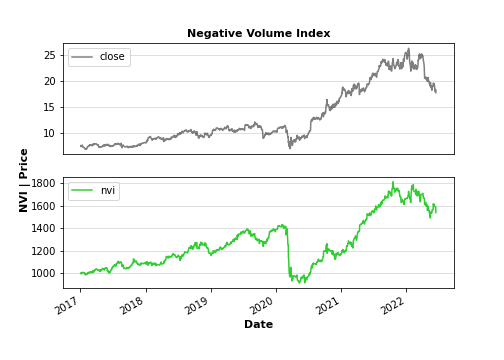
Graph for the calculated fo indicator data, saved.

Simulation Data:
            signal open_trading_action stock_value    exposure portfolio_value  \
Date
2017-01-03   hold                none        7.37         0.0             0.0
2017-01-04   hold                none       7.565         0.0             0.0
2017-01-05   hold                none        7.51         0.0             0.0
2017-01-06   hold                none        7.41         0.0             0.0
2017-01-09   hold                none        7.48         0.0             0.0
...           ...                 ...         ...         ...             ...
2022-06-10   hold                none       18.33  418.209999      329.939999
2022-06-13   hold                none       17.85  418.209999      321.300007
2022-06-14   hold                none       18.24  418.209999      328.319996
2022-06-15   hold                none   18.290001  418.209999      329.220016
2022-06-16   hold                none       17.67  418.209999      318.060001

              earnings     balance
Date
2017-01-03         0.0         0.0
2017-01-04         0.0         0.0
2017-01-05         0.0         0.0
2017-01-06         0.0         0.0
2017-01-09         0.0         0.0
...                ...         ...
2022-06-10  157.949995  487.889994
2022-06-13  157.949995  479.250002
2022-06-14  157.949995  486.269991
2022-06-15  157.949995  487.170012
2022-06-16  157.949995  476.009996

[1374 rows x 7 columns]

Simulation Statistics:
 {'number_of_trading_days': 1374, 'number_of_buy_signals': 928, 'number_of_ignored_buy_signals': 0, 'number_of_sell_signals': 0, 'number_of_ignored_sell_signals': 0, 'last_stock_value': 17.67, 'last_exposure': 418.21, 'last_open_long_positions': 18, 'last_open_short_positions': 0, 'last_portfolio_value': 318.06, 'last_earnings': 157.95, 'final_balance': 476.01}

Graph for the executed trading signal simulation, saved.
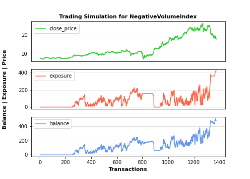
Let’s look at the On-balance volume (OBV) – a simple accumulation-distribution tool that tallies up and down volume, creating a smooth indicator line to predict when major market moves might occur based on changes in relative trading volume.
from tti.indicators import OnBalanceVolume
obv_indicator = OnBalanceVolume(input_data=df)
Get indicator’s value for a specific date
print(‘\nTechnical Indicator value at 2022-06-15:’, obv_indicator.getTiValue(‘2022-06-15’))
Get the most recent indicator’s value
print(‘\nMost recent Technical Indicator value:’, obv_indicator.getTiValue())
Get signal from indicator
print(‘\nTechnical Indicator signal:’, obv_indicator.getTiSignal())
Show the Graph for the calculated Technical Indicator
obv_indicator.getTiGraph().show()
Save the Graph for the calculated Technical Indicator
obv_indicator.getTiGraph().savefig(‘../TTI/example_obv.png’)
print(‘\nGraph for the calculated fo indicator data, saved.’)
Execute simulation based on trading signals
simulation_data, simulation_statistics, simulation_graph = \
obv_indicator.getTiSimulation(
close_values=df[[‘close’]], max_exposure=None,
short_exposure_factor=1.5)
print(‘\nSimulation Data:\n’, simulation_data)
print(‘\nSimulation Statistics:\n’, simulation_statistics)
Save the Graph for the executed trading signal simulation
simulation_graph.savefig(../TTI/simulation_obv.png’)
print(‘\nGraph for the executed trading signal simulation, saved.’)
Technical Indicator value at 2022-06-15: [369390600]

Most recent Technical Indicator value: [363580200]

Technical Indicator signal: ('hold', 0)

Graph for the calculated fo indicator data, saved.

Simulation Data:
            signal open_trading_action stock_value    exposure portfolio_value  \
Date
2017-01-03   hold                none        7.37         0.0             0.0
2017-01-04   hold                none       7.565         0.0             0.0
2017-01-05   hold                none        7.51         0.0             0.0
2017-01-06    buy                long        7.41        7.41            7.41
2017-01-09   hold                none        7.48         0.0             0.0
...           ...                 ...         ...         ...             ...
2022-06-10    buy                long       18.33  497.329997             0.0
2022-06-13    buy                long       17.85  515.179997           17.85
2022-06-14   hold                none       18.24  497.329997             0.0
2022-06-15   sell               short   18.290001  524.764998      -18.290001
2022-06-16   hold                none       17.67  497.329997             0.0

             earnings     balance
Date
2017-01-03        0.0         0.0
2017-01-04        0.0         0.0
2017-01-05        0.0         0.0
2017-01-06        0.0        7.41
2017-01-09       0.07        0.07
...               ...         ...
2022-06-10  98.119987   98.119987
2022-06-13  98.119987  115.969987
2022-06-14  98.509986   98.509986
2022-06-15  98.509986   80.219985
2022-06-16  99.129987   99.129987

[1374 rows x 7 columns]

Simulation Statistics:
 {'number_of_trading_days': 1374, 'number_of_buy_signals': 281, 'number_of_ignored_buy_signals': 0, 'number_of_sell_signals': 370, 'number_of_ignored_sell_signals': 0, 'last_stock_value': 17.67, 'last_exposure': 497.33, 'last_open_long_positions': 13, 'last_open_short_positions': 13, 'last_portfolio_value': 0.0, 'last_earnings': 99.13, 'final_balance': 99.13}

Graph for the executed trading signal simulation, saved.

Let’s look at the parabolic SAR (PSAR) trading strategy. It is essentially a trend trading strategy. It is used to identify a particular trend, and it attempts to forecast trend continuations and potential trend reversals. For example, if the parabolic line is green, you would follow the bullish trend and keep your long position open.
from tti.indicators import ParabolicSAR
psar_indicator = ParabolicSAR(input_data=df)
Get indicator’s value for a specific date
print(‘\nTechnical Indicator value at 2022-06-15:’, psar_indicator.getTiValue(‘2022-06-15’))
Get the most recent indicator’s value
print(‘\nMost recent Technical Indicator value:’, psar_indicator.getTiValue())
Get signal from indicator
print(‘\nTechnical Indicator signal:’, psar_indicator.getTiSignal())
Show the Graph for the calculated Technical Indicator
psar_indicator.getTiGraph().show()
Save the Graph for the calculated Technical Indicator
psar_indicator.getTiGraph().savefig(‘../TTI/example_psar.png’)
print(‘\nGraph for the calculated fo indicator data, saved.’)
Execute simulation based on trading signals
simulation_data, simulation_statistics, simulation_graph = \
psar_indicator.getTiSimulation(
close_values=df[[‘close’]], max_exposure=None,
short_exposure_factor=1.5)
print(‘\nSimulation Data:\n’, simulation_data)
print(‘\nSimulation Statistics:\n’, simulation_statistics)
Save the Graph for the executed trading signal simulation
simulation_graph.savefig(‘../TTI/simulation_psar.png’)
print(‘\nGraph for the executed trading signal simulation, saved.’)
Technical Indicator value at 2022-06-15: [19.4661]

Most recent Technical Indicator value: [19.3978]

Technical Indicator signal: ('hold', 0)

Graph for the calculated fo indicator data, saved.

Simulation Data:
            signal open_trading_action stock_value   exposure portfolio_value  \
Date
2017-01-03   hold                none        7.37        0.0             0.0
2017-01-04   hold                none       7.565        0.0             0.0
2017-01-05   hold                none        7.51        0.0             0.0
2017-01-06    buy                long        7.41       7.41            7.41
2017-01-09   hold                none        7.48        0.0             0.0
...           ...                 ...         ...        ...             ...
2022-06-10    buy                long       18.33  62.559999           54.99
2022-06-13   hold                none       17.85  62.559999       53.550001
2022-06-14   hold                none       18.24  62.559999       54.719999
2022-06-15   hold                none   18.290001  62.559999       54.870003
2022-06-16   hold                none       17.67  62.559999           53.01

             earnings    balance
Date
2017-01-03        0.0        0.0
2017-01-04        0.0        0.0
2017-01-05        0.0        0.0
2017-01-06        0.0       7.41
2017-01-09       0.07       0.07
...               ...        ...
2022-06-10  20.339995  75.329995
2022-06-13  20.339995  73.889996
2022-06-14  20.339995  75.059994
2022-06-15  20.339995  75.209998
2022-06-16  20.339995  73.349995

[1374 rows x 7 columns]

Simulation Statistics:
 {'number_of_trading_days': 1374, 'number_of_buy_signals': 58, 'number_of_ignored_buy_signals': 0, 'number_of_sell_signals': 57, 'number_of_ignored_sell_signals': 0, 'last_stock_value': 17.67, 'last_exposure': 62.56, 'last_open_long_positions': 3, 'last_open_short_positions': 0, 'last_portfolio_value': 53.01, 'last_earnings': 20.34, 'final_balance': 73.35}

Graph for the executed trading signal simulation, saved.

Let’s check the Performance (PERF) indicator. In stock market, performance indicator is a technical indicator used to indicate rate of change of a stock over a specified time period. Observing stock market performance is significant for traders to make trading decisions.
from tti.indicators import Performance
perf_indicator = Performance(input_data=df)
Get indicator’s value for a specific date
print(‘\nTechnical Indicator value at 2022-06-15:’, perf_indicator.getTiValue(‘2022-06-15’))
Get the most recent indicator’s value
print(‘\nMost recent Technical Indicator value:’, perf_indicator.getTiValue())
Get signal from indicator
print(‘\nTechnical Indicator signal:’, perf_indicator.getTiSignal())
Show the Graph for the calculated Technical Indicator
perf_indicator.getTiGraph().show()
Save the Graph for the calculated Technical Indicator
perf_indicator.getTiGraph().savefig(‘../TTI/example_perf.png’)
print(‘\nGraph for the calculated fo indicator data, saved.’)
Execute simulation based on trading signals
simulation_data, simulation_statistics, simulation_graph = \
perf_indicator.getTiSimulation(
close_values=df[[‘close’]], max_exposure=None,
short_exposure_factor=1.5)
print(‘\nSimulation Data:\n’, simulation_data)
print(‘\nSimulation Statistics:\n’, simulation_statistics)
Save the Graph for the executed trading signal simulation
simulation_graph.savefig(‘../TTI/simulation_perf.png’)
print(‘\nGraph for the executed trading signal simulation, saved.’)
Technical Indicator value at 2022-06-15: [1.4817, 0.05]

Most recent Technical Indicator value: [1.3976, 0.05]

Technical Indicator signal: ('sell', 1)
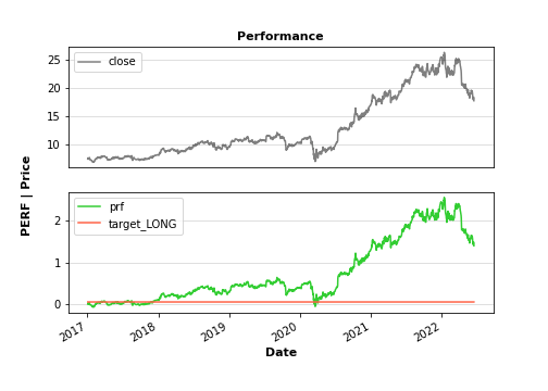
Graph for the calculated fo indicator data, saved.

Simulation Data:
            signal open_trading_action stock_value     exposure  \
Date
2017-01-03   hold                none        7.37          0.0
2017-01-04   hold                none       7.565          0.0
2017-01-05   hold                none        7.51          0.0
2017-01-06   hold                none        7.41          0.0
2017-01-09   hold                none        7.48          0.0
...           ...                 ...         ...          ...
2022-06-10   sell               short       18.33  1048.094998
2022-06-13   sell               short       17.85   993.345001
2022-06-14   sell               short       18.24     1020.705
2022-06-15   sell               short   18.290001  1048.140002
2022-06-16   sell               short       17.67      966.315

           portfolio_value    earnings     balance
Date
2017-01-03             0.0         0.0         0.0
2017-01-04             0.0         0.0         0.0
2017-01-05             0.0         0.0         0.0
2017-01-06             0.0         0.0         0.0
2017-01-09             0.0         0.0         0.0
...                    ...         ...         ...
2022-06-10     -989.819996  203.429988 -786.390008
2022-06-13      -928.20002  204.229985 -723.970035
2022-06-14     -966.719988  204.229985 -762.490003
2022-06-15     -987.660049  204.229985 -783.430064
2022-06-16     -901.170004  205.769986 -695.400018

[1374 rows x 7 columns]

Simulation Statistics:
 {'number_of_trading_days': 1374, 'number_of_buy_signals': 0, 'number_of_ignored_buy_signals': 0, 'number_of_sell_signals': 1181, 'number_of_ignored_sell_signals': 0, 'last_stock_value': 17.67, 'last_exposure': 966.32, 'last_open_long_positions': 0, 'last_open_short_positions': 51, 'last_portfolio_value': -901.17, 'last_earnings': 205.77, 'final_balance': -695.4}

Graph for the executed trading signal simulation, saved.
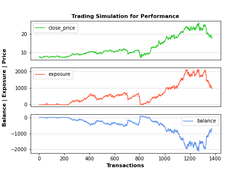
Let’s look at the Positive Volume Index (PVI). PVI is often used in conjunction with the Negative Volume Index (NVI) to identify bull and bear markets. The PVI focuses on days when the volume has increased from the previous day. PVI’s premise is that the “uninformed crowd” takes positions on days when volume increases.
from tti.indicators import PositiveVolumeIndex
pvi_indicator = PositiveVolumeIndex(input_data=df)
Get indicator’s value for a specific date
print(‘\nTechnical Indicator value at 2022-06-15:’, pvi_indicator.getTiValue(‘2022-06-15’))
Get the most recent indicator’s value
print(‘\nMost recent Technical Indicator value:’, pvi_indicator.getTiValue())
Get signal from indicator
print(‘\nTechnical Indicator signal:’, pvi_indicator.getTiSignal())
Show the Graph for the calculated Technical Indicator
pvi_indicator.getTiGraph().show()
Save the Graph for the calculated Technical Indicator
pvi_indicator.getTiGraph().savefig(‘../TTI/example_pvi.png’)
print(‘\nGraph for the calculated fo indicator data, saved.’)
Execute simulation based on trading signals
simulation_data, simulation_statistics, simulation_graph = \
pvi_indicator.getTiSimulation(
close_values=df[[‘close’]], max_exposure=None,
short_exposure_factor=1.5)
print(‘\nSimulation Data:\n’, simulation_data)
print(‘\nSimulation Statistics:\n’, simulation_statistics)
Save the Graph for the executed trading signal simulation
simulation_graph.savefig(‘../TTI/simulation_pvi.png’)
print(‘\nGraph for the executed trading signal simulation, saved.’)
Technical Indicator value at 2022-06-15: [1557.8031]

Most recent Technical Indicator value: [1557.8031]

Technical Indicator signal: ('hold', 0)

Graph for the calculated fo indicator data, saved.

Simulation Data:
            signal open_trading_action stock_value exposure portfolio_value  \
Date
2017-01-03   hold                none        7.37      0.0             0.0
2017-01-04   hold                none       7.565      0.0             0.0
2017-01-05   hold                none        7.51      0.0             0.0
2017-01-06   hold                none        7.41      0.0             0.0
2017-01-09   hold                none        7.48      0.0             0.0
...           ...                 ...         ...      ...             ...
2022-06-10   hold                none       18.33    26.76          -18.33
2022-06-13   hold                none       17.85    26.76          -17.85
2022-06-14   hold                none       18.24    26.76          -18.24
2022-06-15   hold                none   18.290001    26.76      -18.290001
2022-06-16   hold                none       17.67      0.0             0.0

           earnings    balance
Date
2017-01-03      0.0        0.0
2017-01-04      0.0        0.0
2017-01-05      0.0        0.0
2017-01-06      0.0        0.0
2017-01-09      0.0        0.0
...             ...        ...
2022-06-10    7.005    -11.325
2022-06-13    7.005 -10.845001
2022-06-14    7.005    -11.235
2022-06-15    7.005 -11.285001
2022-06-16    7.175      7.175

[1374 rows x 7 columns]

Simulation Statistics:
 {'number_of_trading_days': 1374, 'number_of_buy_signals': 15, 'number_of_ignored_buy_signals': 0, 'number_of_sell_signals': 16, 'number_of_ignored_sell_signals': 0, 'last_stock_value': 17.67, 'last_exposure': 0.0, 'last_open_long_positions': 0, 'last_open_short_positions': 0, 'last_portfolio_value': 0.0, 'last_earnings': 7.17, 'final_balance': 7.17}

Graph for the executed trading signal simulation, saved.

Let’s consider the Price And Volume Trend (PVT).
The volume price trend indicator is used to determine the balance between a security’s demand and supply. The percentage change in the share price trend shows the relative supply or demand of a particular security, while volume indicates the force behind the trend.
from tti.indicators import PriceAndVolumeTrend
pvt_indicator = PriceAndVolumeTrend(input_data=df)
Get indicator’s value for a specific date
print(‘\nTechnical Indicator value at 2022-06-15:’, pvt_indicator.getTiValue(‘2022-06-15’))
Get the most recent indicator’s value
print(‘\nMost recent Technical Indicator value:’, pvt_indicator.getTiValue())
Get signal from indicator
print(‘\nTechnical Indicator signal:’, pvt_indicator.getTiSignal())
Show the Graph for the calculated Technical Indicator
pvt_indicator.getTiGraph().show()
Save the Graph for the calculated Technical Indicator
pvt_indicator.getTiGraph().savefig(‘../TTI/example_pvt.png’)
print(‘\nGraph for the calculated fo indicator data, saved.’)
Execute simulation based on trading signals
simulation_data, simulation_statistics, simulation_graph = \
pvt_indicator.getTiSimulation(
close_values=df[[‘close’]], max_exposure=None,
short_exposure_factor=1.5)
print(‘\nSimulation Data:\n’, simulation_data)
print(‘\nSimulation Statistics:\n’, simulation_statistics)
Save the Graph for the executed trading signal simulation
simulation_graph.savefig(‘../TTI/simulation_pvt.png’)
print(‘\nGraph for the executed trading signal simulation, saved.’)
Technical Indicator value at 2022-06-15: [-1649913.889]

Most recent Technical Indicator value: [-1846876.8576]

Technical Indicator signal: ('hold', 0)
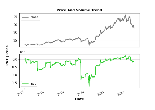
Graph for the calculated fo indicator data, saved.

Simulation Data:
            signal open_trading_action stock_value    exposure portfolio_value  \
Date
2017-01-03   hold                none        7.37         0.0             0.0
2017-01-04   hold                none       7.565         0.0             0.0
2017-01-05   hold                none        7.51         0.0             0.0
2017-01-06    buy                long        7.41        7.41            7.41
2017-01-09   hold                none        7.48         0.0             0.0
...           ...                 ...         ...         ...             ...
2022-06-10    buy                long       18.33  497.329997             0.0
2022-06-13    buy                long       17.85  515.179997           17.85
2022-06-14   hold                none       18.24  497.329997             0.0
2022-06-15   sell               short   18.290001  524.764998      -18.290001
2022-06-16   hold                none       17.67  497.329997             0.0

             earnings     balance
Date
2017-01-03        0.0         0.0
2017-01-04        0.0         0.0
2017-01-05        0.0         0.0
2017-01-06        0.0        7.41
2017-01-09       0.07        0.07
...               ...         ...
2022-06-10  98.119987   98.119987
2022-06-13  98.119987  115.969987
2022-06-14  98.509986   98.509986
2022-06-15  98.509986   80.219985
2022-06-16  99.129987   99.129987

[1374 rows x 7 columns]

Simulation Statistics:
 {'number_of_trading_days': 1374, 'number_of_buy_signals': 281, 'number_of_ignored_buy_signals': 0, 'number_of_sell_signals': 370, 'number_of_ignored_sell_signals': 0, 'last_stock_value': 17.67, 'last_exposure': 497.33, 'last_open_long_positions': 13, 'last_open_short_positions': 13, 'last_portfolio_value': 0.0, 'last_earnings': 99.13, 'final_balance': 99.13}

Graph for the executed trading signal simulation, saved.

Let’s look at the Price Channel Strategy. It was created for breakdowns and breakouts from specific channels. This strategy can be used by momentum traders or swing traders who are looking to detect breakouts from specific ranges. The strategy creates a channel with its bands based on the highest and lowest values for a specific number of bars.
from tti.indicators import PriceChannel
pch_indicator = PriceChannel(input_data=df)
Get indicator’s value for a specific date
print(‘\nTechnical Indicator value at 2022-06-15:’, pch_indicator.getTiValue(‘2022-06-15’))
Get the most recent indicator’s value
print(‘\nMost recent Technical Indicator value:’, pch_indicator.getTiValue())
Get signal foom indicator
print(‘\nTechnical Indicator signal:’, pch_indicator.getTiSignal())
Show the Graph for the calculated Technical Indicator
pch_indicator.getTiGraph().show()
Save the Graph for the calculated Technical Indicator
pch_indicator.getTiGraph().savefig(‘../TTI/example_pch.png’)
print(‘\nGraph for the calculated fo indicator data, saved.’)
Execute simulation based on trading signals
simulation_data, simulation_statistics, simulation_graph = \
pch_indicator.getTiSimulation(
close_values=df[[‘close’]], max_exposure=None,
short_exposure_factor=1.5)
print(‘\nSimulation Data:\n’, simulation_data)
print(‘\nSimulation Statistics:\n’, simulation_statistics)
Save the Graph for the executed trading signal simulation
simulation_graph.savefig(‘../TTI/simulation_pch.png’)
print(‘\nGraph for the executed trading signal simulation, saved.’)
Technical Indicator value at 2022-06-15: [19.31, 17.76]

Most recent Technical Indicator value: [19.29, 17.76]

Technical Indicator signal: ('buy', -1)
Graph for the calculated fo indicator data, saved.

Simulation Data:
            signal open_trading_action stock_value    exposure portfolio_value  \
Date
2017-01-03   hold                none        7.37         0.0             0.0
2017-01-04   hold                none       7.565         0.0             0.0
2017-01-05   hold                none        7.51         0.0             0.0
2017-01-06   hold                none        7.41         0.0             0.0
2017-01-09   hold                none        7.48         0.0             0.0
...           ...                 ...         ...         ...             ...
2022-06-10    buy                long       18.33  259.199996           18.33
2022-06-13    buy                long       17.85  277.049996       35.700001
2022-06-14   hold                none       18.24  259.199996           18.24
2022-06-15   hold                none   18.290001  259.199996       18.290001
2022-06-16    buy                long       17.67  276.869996           35.34

             earnings     balance
Date
2017-01-03        0.0         0.0
2017-01-04        0.0         0.0
2017-01-05        0.0         0.0
2017-01-06        0.0         0.0
2017-01-09        0.0         0.0
...               ...         ...
2022-06-10  64.709998   83.039998
2022-06-13  64.709998  100.409998
2022-06-14  65.099997   83.339997
2022-06-15  65.099997   83.389998
2022-06-16  65.099997  100.439997

[1374 rows x 7 columns]

Simulation Statistics:
 {'number_of_trading_days': 1374, 'number_of_buy_signals': 152, 'number_of_ignored_buy_signals': 0, 'number_of_sell_signals': 222, 'number_of_ignored_sell_signals': 0, 'last_stock_value': 17.67, 'last_exposure': 276.87, 'last_open_long_positions': 8, 'last_open_short_positions': 6, 'last_portfolio_value': 35.34, 'last_earnings': 65.1, 'final_balance': 100.44}

Graph for the executed trading signal simulation, saved.

Let’s calculate the price oscillator (PO) – a technical momentum indicator that shows the relationship between two moving averages in percentage terms. The moving averages are a 26-period and 12-period exponential moving average (EMA).
from tti.indicators import PriceOscillator
posc_indicator = PriceOscillator(input_data=df)
Get indicator’s value for a specific date
print(‘\nTechnical Indicator value at 2022-06-15:’, posc_indicator.getTiValue(‘2022-06-15’))
Get the most recent indicator’s value
print(‘\nMost recent Technical Indicator value:’, posc_indicator.getTiValue())
Get signal from indicator
print(‘\nTechnical Indicator signal:’, posc_indicator.getTiSignal())
Show the Graph for the calculated Technical Indicator
posc_indicator.getTiGraph().show()
Save the Graph for the calculated Technical Indicator
posc_indicator.getTiGraph().savefig(‘../TTI/example_posc.png’)
print(‘\nGraph for the calculated fo indicator data, saved.’)
Execute simulation based on trading signals
simulation_data, simulation_statistics, simulation_graph = \
posc_indicator.getTiSimulation(
close_values=df[[‘close’]], max_exposure=None,
short_exposure_factor=1.5)
print(‘\nSimulation Data:\n’, simulation_data)
print(‘\nSimulation Statistics:\n’, simulation_statistics)
Save the Graph for the executed trading signal simulation
simulation_graph.savefig(‘../TTI/simulation_posc.png’)
print(‘\nGraph for the executed trading signal simulation, saved.’)
Technical Indicator value at 2022-06-15: [-1.2696]

Most recent Technical Indicator value: [-1.729]

Technical Indicator signal: ('hold', 0)

Graph for the calculated fo indicator data, saved.

Simulation Data:
            signal open_trading_action stock_value exposure portfolio_value  \
Date
2017-01-03   hold                none        7.37      0.0             0.0
2017-01-04   hold                none       7.565      0.0             0.0
2017-01-05   hold                none        7.51      0.0             0.0
2017-01-06   hold                none        7.41      0.0             0.0
2017-01-09   hold                none        7.48      0.0             0.0
...           ...                 ...         ...      ...             ...
2022-06-10   hold                none       18.33      0.0             0.0
2022-06-13   hold                none       17.85      0.0             0.0
2022-06-14   hold                none       18.24      0.0             0.0
2022-06-15   hold                none   18.290001      0.0             0.0
2022-06-16   hold                none       17.67      0.0             0.0

            earnings   balance
Date
2017-01-03       0.0       0.0
2017-01-04       0.0       0.0
2017-01-05       0.0       0.0
2017-01-06       0.0       0.0
2017-01-09       0.0       0.0
...              ...       ...
2022-06-10  7.334997  7.334997
2022-06-13  7.334997  7.334997
2022-06-14  7.334997  7.334997
2022-06-15  7.334997  7.334997
2022-06-16  7.334997  7.334997

[1374 rows x 7 columns]

Simulation Statistics:
 {'number_of_trading_days': 1374, 'number_of_buy_signals': 23, 'number_of_ignored_buy_signals': 0, 'number_of_sell_signals': 23, 'number_of_ignored_sell_signals': 0, 'last_stock_value': 17.67, 'last_exposure': 0.0, 'last_open_long_positions': 0, 'last_open_short_positions': 0, 'last_portfolio_value': 0.0, 'last_earnings': 7.33, 'final_balance': 7.33}

Graph for the executed trading signal simulation, saved.
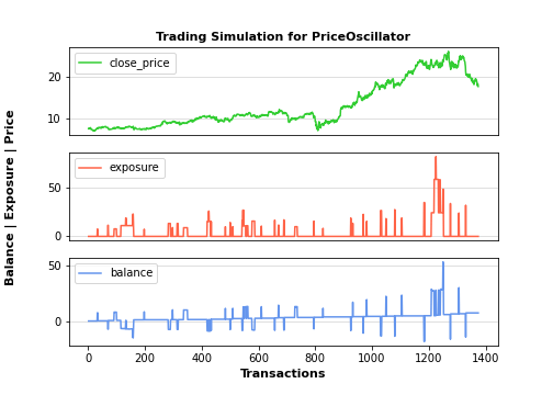
It is interesting to consider the Price Rate of Change (ROC) – a momentum-based technical indicator that measures the percentage change in price between the current price and the price a certain number of periods ago. The ROC indicator is plotted against zero, with the indicator moving upwards into positive territory if price changes are to the upside, and moving into negative territory if price changes are to the downside.
The indicator can be used to spot divergences, overbought and oversold conditions, and centerline crossovers.
from tti.indicators import PriceRateOfChange
proc_indicator = PriceRateOfChange(input_data=df)
Get indicator’s value for a specific date
print(‘\nTechnical Indicator value at 2022-06-15:’, proc_indicator.getTiValue(‘2022-06-15’))
Get the most recent indicator’s value
print(‘\nMost recent Technical Indicator value:’, proc_indicator.getTiValue())
Get signal from indicator
print(‘\nTechnical Indicator signal:’, proc_indicator.getTiSignal())
Show the Graph for the calculated Technical Indicator
proc_indicator.getTiGraph().show()
Save the Graph for the calculated Technical Indicator
proc_indicator.getTiGraph().savefig(‘../TTI/example_proc.png’)
print(‘\nGraph for the calculated fo indicator data, saved.’)
Execute simulation based on trading signals
simulation_data, simulation_statistics, simulation_graph = \
proc_indicator.getTiSimulation(
close_values=df[[‘close’]], max_exposure=None,
short_exposure_factor=1.5)
print(‘\nSimulation Data:\n’, simulation_data)
print(‘\nSimulation Statistics:\n’, simulation_statistics)
Save the Graph for the executed trading signal simulation
simulation_graph.savefig(‘../TTI/simulation_proc.png’)
print(‘\nGraph for the executed trading signal simulation, saved.’)
Technical Indicator value at 2022-06-15: [-7.4393]

Most recent Technical Indicator value: [-8.9645]

Technical Indicator signal: ('hold', 0)

Graph for the calculated fo indicator data, saved.

Simulation Data:
            signal open_trading_action stock_value    exposure portfolio_value  \
Date
2017-01-03   hold                none        7.37         0.0             0.0
2017-01-04   hold                none       7.565         0.0             0.0
2017-01-05   hold                none        7.51         0.0             0.0
2017-01-06   hold                none        7.41         0.0             0.0
2017-01-09   hold                none        7.48         0.0             0.0
...           ...                 ...         ...         ...             ...
2022-06-10    buy                long       18.33  454.744998             0.0
2022-06-13    buy                long       17.85  472.594999           17.85
2022-06-14   hold                none       18.24  454.744998             0.0
2022-06-15   sell               short   18.290001      482.18      -18.290001
2022-06-16   hold                none       17.67  454.744998             0.0

             earnings     balance
Date
2017-01-03        0.0         0.0
2017-01-04        0.0         0.0
2017-01-05        0.0         0.0
2017-01-06        0.0         0.0
2017-01-09        0.0         0.0
...               ...         ...
2022-06-10  91.494991   91.494991
2022-06-13  91.494991  109.344991
2022-06-14   91.88499    91.88499
2022-06-15   91.88499   73.594989
2022-06-16  92.504991   92.504991

[1374 rows x 7 columns]

Simulation Statistics:
 {'number_of_trading_days': 1374, 'number_of_buy_signals': 332, 'number_of_ignored_buy_signals': 0, 'number_of_sell_signals': 308, 'number_of_ignored_sell_signals': 0, 'last_stock_value': 17.67, 'last_exposure': 454.74, 'last_open_long_positions': 11, 'last_open_short_positions': 11, 'last_portfolio_value': 0.0, 'last_earnings': 92.5, 'final_balance': 92.5}

Graph for the executed trading signal simulation, saved.
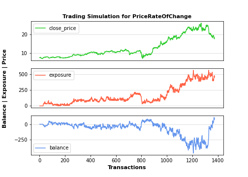
Let’s plot the Projection Bands (PBS). PBS are drawn by finding the minimum and maximum prices over a specified number of days and projecting these forward, parallel to a linear regression line. The resulting plot consists of two bands representing the minimum and maximum price boundaries.
from tti.indicators import ProjectionBands
projb_indicator = ProjectionBands(input_data=df)
Get indicator’s value for a specific date
print(‘\nTechnical Indicator value at 2022-06-15:’, projb_indicator.getTiValue(‘2022-06-15’))
Get the most recent indicator’s value
print(‘\nMost recent Technical Indicator value:’, projb_indicator.getTiValue())
Get signal from indicator
print(‘\nTechnical Indicator signal:’, projb_indicator.getTiSignal())
Show the Graph for the calculated Technical Indicator
projb_indicator.getTiGraph().show()
Save the Graph for the calculated Technical Indicator
projb_indicator.getTiGraph().savefig(‘../TTI/example_projb.png’)
print(‘\nGraph for the calculated fo indicator data, saved.’)
Execute simulation based on trading signals
simulation_data, simulation_statistics, simulation_graph = \
projb_indicator.getTiSimulation(
close_values=df[[‘close’]], max_exposure=None,
short_exposure_factor=1.5)
print(‘\nSimulation Data:\n’, simulation_data)
print(‘\nSimulation Statistics:\n’, simulation_statistics)
Save the Graph for the executed trading signal simulation
simulation_graph.savefig(‘../TTI/simulation_projb.png’)
print(‘\nGraph for the executed trading signal simulation, saved.’)
Technical Indicator value at 2022-06-15: [19.2262, 17.372]

Most recent Technical Indicator value: [18.7765, 17.3609]

Technical Indicator signal: ('hold', 0)
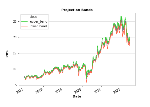
Graph for the calculated fo indicator data, saved.

Simulation Data:
            signal open_trading_action stock_value    exposure portfolio_value  \
Date
2017-01-03   hold                none        7.37         0.0             0.0
2017-01-04   hold                none       7.565         0.0             0.0
2017-01-05   hold                none        7.51         0.0             0.0
2017-01-06   hold                none        7.41         0.0             0.0
2017-01-09   hold                none        7.48         0.0             0.0
...           ...                 ...         ...         ...             ...
2022-06-10    buy                long       18.33  204.944997          109.98
2022-06-13    buy                long       17.85  222.794998      124.950003
2022-06-14   hold                none       18.24  204.944997      109.439999
2022-06-15   hold                none   18.290001  204.944997      109.740005
2022-06-16   hold                none       17.67  204.944997          106.02

             earnings     balance
Date
2017-01-03        0.0         0.0
2017-01-04        0.0         0.0
2017-01-05        0.0         0.0
2017-01-06        0.0         0.0
2017-01-09        0.0         0.0
...               ...         ...
2022-06-10  53.154989  163.134989
2022-06-13  53.154989  178.104992
2022-06-14  53.544989  162.984987
2022-06-15  53.544989  163.284994
2022-06-16  53.544989  159.564989

[1374 rows x 7 columns]

Simulation Statistics:
 {'number_of_trading_days': 1374, 'number_of_buy_signals': 169, 'number_of_ignored_buy_signals': 0, 'number_of_sell_signals': 151, 'number_of_ignored_sell_signals': 0, 'last_stock_value': 17.67, 'last_exposure': 204.94, 'last_open_long_positions': 8, 'last_open_short_positions': 2, 'last_portfolio_value': 106.02, 'last_earnings': 53.54, 'final_balance': 159.56}

Graph for the executed trading signal simulation, saved.
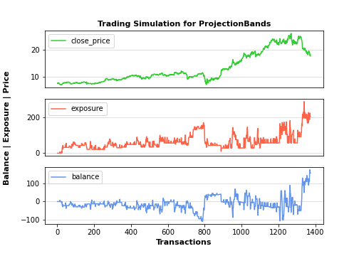
Let’s look at the Projection Oscillator study shows the relationship between the current price and its minimum and maximum prices over time. Unlike the Stochastic Oscillator, here the minimum and maximum prices are adjusted up or down by the slope of the price’s regression line.
from tti.indicators import ProjectionOscillator
projosc_indicator = ProjectionOscillator(input_data=df)
Get indicator’s value for a specific date
print(‘\nTechnical Indicator value at 2022-06-15:’, projosc_indicator.getTiValue(‘2022-06-15’))
Get the most recent indicator’s value
print(‘\nMost recent Technical Indicator value:’, projosc_indicator.getTiValue())
Get signal from indicator
print(‘\nTechnical Indicator signal:’, projosc_indicator.getTiSignal())
Show the Graph for the calculated Technical Indicator
projosc_indicator.getTiGraph().show()
Save the Graph for the calculated Technical Indicator
projosc_indicator.getTiGraph().savefig(‘../TTI/example_projosc.png’)
print(‘\nGraph for the calculated fo indicator data, saved.’)
Execute simulation based on trading signals
simulation_data, simulation_statistics, simulation_graph = \
projosc_indicator.getTiSimulation(
close_values=df[[‘close’]], max_exposure=None,
short_exposure_factor=1.5)
print(‘\nSimulation Data:\n’, simulation_data)
print(‘\nSimulation Statistics:\n’, simulation_statistics)
Save the Graph for the executed trading signal simulation
simulation_graph.savefig(‘../TTI/simulation_projosc.png’)
print(‘\nGraph for the executed trading signal simulation, saved.’)
Technical Indicator value at 2022-06-15: [49.5093, 34.7614]

Most recent Technical Indicator value: [21.8353, 28.2983]

Technical Indicator signal: ('hold', 0)

Graph for the calculated fo indicator data, saved.

Simulation Data:
            signal open_trading_action stock_value    exposure portfolio_value  \
Date
2017-01-03   hold                none        7.37         0.0             0.0
2017-01-04   hold                none       7.565         0.0             0.0
2017-01-05   hold                none        7.51         0.0             0.0
2017-01-06   hold                none        7.41         0.0             0.0
2017-01-09   hold                none        7.48         0.0             0.0
...           ...                 ...         ...         ...             ...
2022-06-10   hold                none       18.33  177.432501          -91.65
2022-06-13   hold                none       17.85  150.222502      -71.400002
2022-06-14    buy                long       18.24  168.462502      -54.719999
2022-06-15    buy                long   18.290001  168.512503      -54.870003
2022-06-16   hold                none       17.67  168.512503          -53.01

             earnings    balance
Date
2017-01-03        0.0        0.0
2017-01-04        0.0        0.0
2017-01-05        0.0        0.0
2017-01-06        0.0        0.0
2017-01-09        0.0        0.0
...               ...        ...
2022-06-10  57.199993 -34.450006
2022-06-13  57.489992 -13.910009
2022-06-14  57.489992   2.769993
2022-06-15  57.539993   2.669991
2022-06-16  57.539993   4.529993

[1374 rows x 7 columns]

Simulation Statistics:
 {'number_of_trading_days': 1374, 'number_of_buy_signals': 198, 'number_of_ignored_buy_signals': 0, 'number_of_sell_signals': 184, 'number_of_ignored_sell_signals': 0, 'last_stock_value': 17.67, 'last_exposure': 168.51, 'last_open_long_positions': 3, 'last_open_short_positions': 6, 'last_portfolio_value': -53.01, 'last_earnings': 57.54, 'final_balance': 4.53}

Graph for the executed trading signal simulation, saved.

Let’s examine the Qstick indicator – a technical analysis indicator developed by Tushar Chande to numerically identify trends on a price chart. It is calculated by taking an ‘n’ period moving average of the difference between the open and closing prices. A Qstick value greater than zero means that the majority of the last ‘n’ days have been up, indicating that buying pressure has been increasing.
The Qstick Indicator is also called Quick Stick. It is not widely available in trading and charting software.
from tti.indicators import Qstick
qstk_indicator = Qstick(input_data=df)
Get indicator’s value for a specific date
print(‘\nTechnical Indicator value at 2022-06-15:’, qstk_indicator.getTiValue(‘2022-06-15’))
Get the most recent indicator’s value
print(‘\nMost recent Technical Indicator value:’, qstk_indicator.getTiValue())
Get signal from indicator
print(‘\nTechnical Indicator signal:’, qstk_indicator.getTiSignal())
Show the Graph for the calculated Technical Indicator
qstk_indicator.getTiGraph().show()
Save the Graph for the calculated Technical Indicator
qstk_indicator.getTiGraph().savefig(‘C:/Users/adrou/OneDrive/Documents/TTI/example_qstk.png’)
print(‘\nGraph for the calculated fo indicator data, saved.’)
Execute simulation based on trading signals
simulation_data, simulation_statistics, simulation_graph = \
qstk_indicator.getTiSimulation(
close_values=df[[‘close’]], max_exposure=None,
short_exposure_factor=1.5)
print(‘\nSimulation Data:\n’, simulation_data)
print(‘\nSimulation Statistics:\n’, simulation_statistics)
Save the Graph for the executed trading signal simulation
simulation_graph.savefig(‘../TTI/simulation_qstk.png’)
print(‘\nGraph for the executed trading signal simulation, saved.’)
Technical Indicator value at 2022-06-15: [-0.02]

Most recent Technical Indicator value: [-0.02]

Technical Indicator signal: ('hold', 0)
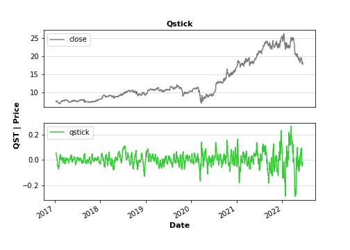
Graph for the calculated fo indicator data, saved.

Simulation Data:
            signal open_trading_action stock_value exposure portfolio_value  \
Date
2017-01-03   hold                none        7.37      0.0             0.0
2017-01-04   hold                none       7.565      0.0             0.0
2017-01-05   hold                none        7.51      0.0             0.0
2017-01-06   hold                none        7.41      0.0             0.0
2017-01-09   hold                none        7.48      0.0             0.0
...           ...                 ...         ...      ...             ...
2022-06-10   sell               short       18.33    96.45          -36.66
2022-06-13   hold                none       17.85   68.955          -17.85
2022-06-14   hold                none       18.24   68.955          -18.24
2022-06-15   hold                none   18.290001   68.955      -18.290001
2022-06-16   hold                none       17.67   68.955          -17.67

             earnings    balance
Date
2017-01-03        0.0        0.0
2017-01-04        0.0        0.0
2017-01-05        0.0        0.0
2017-01-06        0.0        0.0
2017-01-09        0.0        0.0
...               ...        ...
2022-06-10  10.740004 -25.919996
2022-06-13  11.220003  -6.629997
2022-06-14  11.220003  -7.019997
2022-06-15  11.220003  -7.069998
2022-06-16  11.220003  -6.449997

[1374 rows x 7 columns]

Simulation Statistics:
 {'number_of_trading_days': 1374, 'number_of_buy_signals': 34, 'number_of_ignored_buy_signals': 0, 'number_of_sell_signals': 33, 'number_of_ignored_sell_signals': 0, 'last_stock_value': 17.67, 'last_exposure': 68.95, 'last_open_long_positions': 1, 'last_open_short_positions': 2, 'last_portfolio_value': -17.67, 'last_earnings': 11.22, 'final_balance': -6.45}

Graph for the executed trading signal simulation, saved.
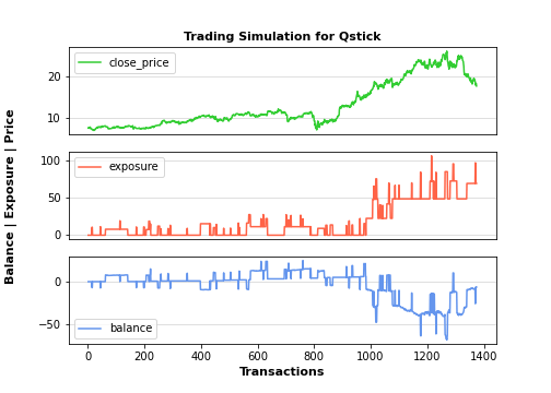
Let’s examine the (true) range indicator taken as the greatest of the following: current high less the current low; the absolute value of the current high less the previous close; and the absolute value of the current low less the previous close.
from tti.indicators import RangeIndicator
rind_indicator = RangeIndicator(input_data=df)
Get indicator’s value for a specific date
print(‘\nTechnical Indicator value at 2022-06-15:’, rind_indicator.getTiValue(‘2022-06-15’))
Get the most recent indicator’s value
print(‘\nMost recent Technical Indicator value:’, rind_indicator.getTiValue())
Get signal from indicator
print(‘\nTechnical Indicator signal:’, rind_indicator.getTiSignal())
Show the Graph for the calculated Technical Indicator
rind_indicator.getTiGraph().show()
Save the Graph for the calculated Technical Indicator
rind_indicator.getTiGraph().savefig(‘../TTI/example_rind.png’)
print(‘\nGraph for the calculated fo indicator data, saved.’)
Execute simulation based on trading signals
simulation_data, simulation_statistics, simulation_graph = \
rind_indicator.getTiSimulation(
close_values=df[[‘close’]], max_exposure=None,
short_exposure_factor=1.5)
print(‘\nSimulation Data:\n’, simulation_data)
print(‘\nSimulation Statistics:\n’, simulation_statistics)
Save the Graph for the executed trading signal simulation
simulation_graph.savefig(‘../TTI/simulation_rind.png’)
print(‘\nGraph for the executed trading signal simulation, saved.’)
Technical Indicator value at 2022-06-15: [85.6335]

Most recent Technical Indicator value: [43.5639]

Technical Indicator signal: ('hold', 0)

Graph for the calculated fo indicator data, saved.

Simulation Data:
            signal open_trading_action stock_value    exposure portfolio_value  \
Date
2017-01-03   hold                none        7.37         0.0             0.0
2017-01-04   hold                none       7.565         0.0             0.0
2017-01-05   hold                none        7.51         0.0             0.0
2017-01-06   hold                none        7.41         0.0             0.0
2017-01-09   hold                none        7.48         0.0             0.0
...           ...                 ...         ...         ...             ...
2022-06-10   hold                none       18.33  103.880001          -36.66
2022-06-13   sell               short       17.85  130.655001      -53.550001
2022-06-14    buy                long       18.24  148.895001          -36.48
2022-06-15   hold                none   18.290001  130.655001      -54.870003
2022-06-16   hold                none       17.67  103.880001          -35.34

             earnings    balance
Date
2017-01-03        0.0        0.0
2017-01-04        0.0        0.0
2017-01-05        0.0        0.0
2017-01-06        0.0        0.0
2017-01-09        0.0        0.0
...               ...        ...
2022-06-10  43.060002   6.400002
2022-06-13  43.060002 -10.489999
2022-06-14  43.060002   6.580003
2022-06-15  43.110003 -11.759999
2022-06-16  43.290004   7.950004

[1374 rows x 7 columns]

Simulation Statistics:
 {'number_of_trading_days': 1374, 'number_of_buy_signals': 188, 'number_of_ignored_buy_signals': 0, 'number_of_sell_signals': 95, 'number_of_ignored_sell_signals': 0, 'last_stock_value': 17.67, 'last_exposure': 103.88, 'last_open_long_positions': 2, 'last_open_short_positions': 4, 'last_portfolio_value': -35.34, 'last_earnings': 43.29, 'final_balance': 7.95}

Graph for the executed trading signal simulation, saved.

Let’s calculate the Relative Momentum Index (RMI) – a variation of the Relative Strength Index (RSI). While the RMI counts up and down days from today’s close relative to the close ”n-days” ago (n is not limited to 1), the RSI counts days up and down from close to close.
from tti.indicators import RelativeMomentumIndex
rmi_indicator = RelativeMomentumIndex(input_data=df)
Get indicator’s value for a specific date
print(‘\nTechnical Indicator value at 2022-06-15:’, rmi_indicator.getTiValue(‘2022-06-15’))
Get the most recent indicator’s value
print(‘\nMost recent Technical Indicator value:’, rmi_indicator.getTiValue())
Get signal from indicator
print(‘\nTechnical Indicator signal:’, rmi_indicator.getTiSignal())
Show the Graph for the calculated Technical Indicator
rmi_indicator.getTiGraph().show()
Save the Graph for the calculated Technical Indicator
rmi_indicator.getTiGraph().savefig(‘../TTI/example_rmi.png’)
print(‘\nGraph for the calculated fo indicator data, saved.’)
Execute simulation based on trading signals
simulation_data, simulation_statistics, simulation_graph = \
rmi_indicator.getTiSimulation(
close_values=df[[‘close’]], max_exposure=None,
short_exposure_factor=1.5)
print(‘\nSimulation Data:\n’, simulation_data)
print(‘\nSimulation Statistics:\n’, simulation_statistics)
Save the Graph for the executed trading signal simulation
simulation_graph.savefig(‘../TTI/simulation_rmi.png’)
print(‘\nGraph for the executed trading signal simulation, saved.’)
Technical Indicator value at 2022-06-15: [21.6699]

Most recent Technical Indicator value: [19.125]

Technical Indicator signal: ('hold', 0)

Graph for the calculated fo indicator data, saved.

Simulation Data:
            signal open_trading_action stock_value   exposure portfolio_value  \
Date
2017-01-03   hold                none        7.37        0.0             0.0
2017-01-04   hold                none       7.565        0.0             0.0
2017-01-05   hold                none        7.51        0.0             0.0
2017-01-06   hold                none        7.41        0.0             0.0
2017-01-09   hold                none        7.48        0.0             0.0
...           ...                 ...         ...        ...             ...
2022-06-10   hold                none       18.33  38.190001             0.0
2022-06-13    buy                long       17.85  56.040001           17.85
2022-06-14   hold                none       18.24  38.190001             0.0
2022-06-15   hold                none   18.290001  38.190001             0.0
2022-06-16   hold                none       17.67  38.190001             0.0

             earnings    balance
Date
2017-01-03        0.0        0.0
2017-01-04        0.0        0.0
2017-01-05        0.0        0.0
2017-01-06        0.0        0.0
2017-01-09        0.0        0.0
...               ...        ...
2022-06-10  11.010005  11.010005
2022-06-13  11.010005  28.860005
2022-06-14  11.400004  11.400004
2022-06-15  11.400004  11.400004
2022-06-16  11.400004  11.400004

[1374 rows x 7 columns]

Simulation Statistics:
 {'number_of_trading_days': 1374, 'number_of_buy_signals': 40, 'number_of_ignored_buy_signals': 0, 'number_of_sell_signals': 49, 'number_of_ignored_sell_signals': 0, 'last_stock_value': 17.67, 'last_exposure': 38.19, 'last_open_long_positions': 1, 'last_open_short_positions': 1, 'last_portfolio_value': 0.0, 'last_earnings': 11.4, 'final_balance': 11.4}

Graph for the executed trading signal simulation, saved.

Let’s look at the relative strength index (RSI) – a momentum indicator used in technical analysis that measures the magnitude of recent price changes to evaluate overbought or oversold conditions in the price of a stock or other asset.
from tti.indicators import RelativeStrengthIndex
rsind_indicator = RelativeStrengthIndex(input_data=df)
Get indicator’s value for a specific date
print(‘\nTechnical Indicator value at 2022-06-15:’, rsind_indicator.getTiValue(‘2022-06-15’))
Get the most recent indicator’s value
print(‘\nMost recent Technical Indicator value:’, rsind_indicator.getTiValue())
Get signal from indicator
print(‘\nTechnical Indicator signal:’, rsind_indicator.getTiSignal())
Show the Graph for the calculated Technical Indicator
rsind_indicator.getTiGraph().show()
Save the Graph for the calculated Technical Indicator
rsind_indicator.getTiGraph().savefig(‘../TTI/example_rsind.png’)
print(‘\nGraph for the calculated fo indicator data, saved.’)
Execute simulation based on trading signals
simulation_data, simulation_statistics, simulation_graph = \
rsind_indicator.getTiSimulation(
close_values=df[[‘close’]], max_exposure=None,
short_exposure_factor=1.5)
print(‘\nSimulation Data:\n’, simulation_data)
print(‘\nSimulation Statistics:\n’, simulation_statistics)
Save the Graph for the executed trading signal simulation
simulation_graph.savefig(‘../TTI/simulation_rsind.png’)
print(‘\nGraph for the executed trading signal simulation, saved.’)
Technical Indicator value at 2022-06-15: [38.6543]

Most recent Technical Indicator value: [33.2274]

Technical Indicator signal: ('hold', 0)

Graph for the calculated fo indicator data, saved.

Simulation Data:
            signal open_trading_action stock_value   exposure portfolio_value  \
Date
2017-01-03   hold                none        7.37        0.0             0.0
2017-01-04   hold                none       7.565        0.0             0.0
2017-01-05   hold                none        7.51        0.0             0.0
2017-01-06   hold                none        7.41        0.0             0.0
2017-01-09   hold                none        7.48        0.0             0.0
...           ...                 ...         ...        ...             ...
2022-06-10   hold                none       18.33  36.895001             0.0
2022-06-13   hold                none       17.85  36.895001             0.0
2022-06-14   hold                none       18.24  36.895001             0.0
2022-06-15   hold                none   18.290001  36.895001             0.0
2022-06-16   hold                none       17.67  36.895001             0.0

           earnings balance
Date
2017-01-03      0.0     0.0
2017-01-04      0.0     0.0
2017-01-05      0.0     0.0
2017-01-06      0.0     0.0
2017-01-09      0.0     0.0
...             ...     ...
2022-06-10     4.75    4.75
2022-06-13     4.75    4.75
2022-06-14     4.75    4.75
2022-06-15     4.75    4.75
2022-06-16     4.75    4.75

[1374 rows x 7 columns]

Simulation Statistics:
 {'number_of_trading_days': 1374, 'number_of_buy_signals': 10, 'number_of_ignored_buy_signals': 0, 'number_of_sell_signals': 24, 'number_of_ignored_sell_signals': 0, 'last_stock_value': 17.67, 'last_exposure': 36.9, 'last_open_long_positions': 1, 'last_open_short_positions': 1, 'last_portfolio_value': 0.0, 'last_earnings': 4.75, 'final_balance': 4.75}

Graph for the executed trading signal simulation, saved.

The Relative Volatility Index (RVI) is similar to the Relative Strength Index (RSI) index. Both measure the direction of volatility, but RVI uses the standard deviation of price changes in its calculations, while RSI uses the absolute price changes.
from tti.indicators import RelativeVolatilityIndex
rvind_indicator = RelativeVolatilityIndex(input_data=df)
Get indicator’s value for a specific date
print(‘\nTechnical Indicator value at 2022-06-15:’, rvind_indicator.getTiValue(‘2022-06-15’))
Get the most recent indicator’s value
print(‘\nMost recent Technical Indicator value:’, rvind_indicator.getTiValue())
Get signal from indicator
print(‘\nTechnical Indicator signal:’, rvind_indicator.getTiSignal())
Show the Graph for the calculated Technical Indicator
rvind_indicator.getTiGraph().show()
Save the Graph for the calculated Technical Indicator
rvind_indicator.getTiGraph().savefig(‘../TTI/example_rvind.png’)
print(‘\nGraph for the calculated fo indicator data, saved.’)
Execute simulation based on trading signals
simulation_data, simulation_statistics, simulation_graph = \
rvind_indicator.getTiSimulation(
close_values=df[[‘close’]], max_exposure=None,
short_exposure_factor=1.5)
print(‘\nSimulation Data:\n’, simulation_data)
print(‘\nSimulation Statistics:\n’, simulation_statistics)
Save the Graph for the executed trading signal simulation
simulation_graph.savefig(‘../TTI/simulation_rvind.png’)
print(‘\nGraph for the executed trading signal simulation, saved.’)
Technical Indicator value at 2022-06-15: [49.6396]

Most recent Technical Indicator value: [36.6158]

Technical Indicator signal: ('buy', -1)
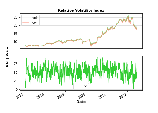
Graph for the calculated fo indicator data, saved.

Simulation Data:
            signal open_trading_action stock_value    exposure portfolio_value  \
Date
2017-01-03   hold                none        7.37         0.0             0.0
2017-01-04   hold                none       7.565         0.0             0.0
2017-01-05   hold                none        7.51         0.0             0.0
2017-01-06   hold                none        7.41         0.0             0.0
2017-01-09   hold                none        7.48         0.0             0.0
...           ...                 ...         ...         ...             ...
2022-06-10   hold                none       18.33  159.864999          -36.66
2022-06-13    buy                long       17.85     177.715          -17.85
2022-06-14   hold                none       18.24  159.864999          -36.48
2022-06-15   hold                none   18.290001  159.864999      -36.580002
2022-06-16    buy                long       17.67  177.534999          -17.67

             earnings    balance
Date
2017-01-03        0.0        0.0
2017-01-04        0.0        0.0
2017-01-05        0.0        0.0
2017-01-06        0.0        0.0
2017-01-09        0.0        0.0
...               ...        ...
2022-06-10  37.405003   0.745003
2022-06-13  37.405003  19.555002
2022-06-14  37.795002   1.315002
2022-06-15  37.795002      1.215
2022-06-16  37.795002  20.125002

[1374 rows x 7 columns]

Simulation Statistics:
 {'number_of_trading_days': 1374, 'number_of_buy_signals': 108, 'number_of_ignored_buy_signals': 0, 'number_of_sell_signals': 130, 'number_of_ignored_sell_signals': 0, 'last_stock_value': 17.67, 'last_exposure': 177.53, 'last_open_long_positions': 4, 'last_open_short_positions': 5, 'last_portfolio_value': -17.67, 'last_earnings': 37.8, 'final_balance': 20.13}

Graph for the executed trading signal simulation, saved.

Next, let’s calculate the Standard Deviation (SD) – a way to measure price volatility by relating a price range to its moving average. The higher the value of the indicator, the wider the spread between price and its moving average, the more volatile the instrument and the more dispersed the price bars become. The lower the value of the indicator, the smaller the spread between price and its moving average, the less volatile the instrument and the closer to each other the price bars become. Standard Deviation is used as part of other indicators such as Bollinger Bands. It is often used in combination with other signals and analysis techniques.
from tti.indicators import StandardDeviation
stdv_indicator = StandardDeviation(input_data=df)
Get indicator’s value for a specific date
print(‘\nTechnical Indicator value at 2022-06-15:’, stdv_indicator.getTiValue(‘2022-06-15’))
Get the most recent indicator’s value
print(‘\nMost recent Technical Indicator value:’, stdv_indicator.getTiValue())
Get signal from indicator
print(‘\nTechnical Indicator signal:’, stdv_indicator.getTiSignal())
Show the Graph for the calculated Technical Indicator
stdv_indicator.getTiGraph().show()
Save the Graph for the calculated Technical Indicator
stdv_indicator.getTiGraph().savefig(‘../TTI/example_stdv.png’)
print(‘\nGraph for the calculated fo indicator data, saved.’)
Execute simulation based on trading signals
simulation_data, simulation_statistics, simulation_graph = \
stdv_indicator.getTiSimulation(
close_values=df[[‘close’]], max_exposure=None,
short_exposure_factor=1.5)
print(‘\nSimulation Data:\n’, simulation_data)
print(‘\nSimulation Statistics:\n’, simulation_statistics)
Save the Graph for the executed trading signal simulation
simulation_graph.savefig(‘../TTI/simulation_stdv.png’)
print(‘\nGraph for the executed trading signal simulation, saved.’)
Technical Indicator value at 2022-06-15: [0.4608]

Most recent Technical Indicator value: [0.519]

Technical Indicator signal: ('hold', 0)

Graph for the calculated fo indicator data, saved.

Simulation Data:
            signal open_trading_action stock_value exposure portfolio_value  \
Date
2017-01-03   hold                none        7.37      0.0             0.0
2017-01-04   hold                none       7.565      0.0             0.0
2017-01-05   hold                none        7.51      0.0             0.0
2017-01-06   hold                none        7.41      0.0             0.0
2017-01-09   hold                none        7.48      0.0             0.0
...           ...                 ...         ...      ...             ...
2022-06-10   hold                none       18.33      0.0             0.0
2022-06-13   hold                none       17.85      0.0             0.0
2022-06-14   hold                none       18.24      0.0             0.0
2022-06-15   hold                none   18.290001      0.0             0.0
2022-06-16   hold                none       17.67      0.0             0.0

           earnings balance
Date
2017-01-03      0.0     0.0
2017-01-04      0.0     0.0
2017-01-05      0.0     0.0
2017-01-06      0.0     0.0
2017-01-09      0.0     0.0
...             ...     ...
2022-06-10      0.0     0.0
2022-06-13      0.0     0.0
2022-06-14      0.0     0.0
2022-06-15      0.0     0.0
2022-06-16      0.0     0.0

[1374 rows x 7 columns]

Simulation Statistics:
 {'number_of_trading_days': 1374, 'number_of_buy_signals': 0, 'number_of_ignored_buy_signals': 0, 'number_of_sell_signals': 0, 'number_of_ignored_sell_signals': 0, 'last_stock_value': 17.67, 'last_exposure': 0.0, 'last_open_long_positions': 0, 'last_open_short_positions': 0, 'last_portfolio_value': 0.0, 'last_earnings': 0.0, 'final_balance': 0.0}

Graph for the executed trading signal simulation, saved.
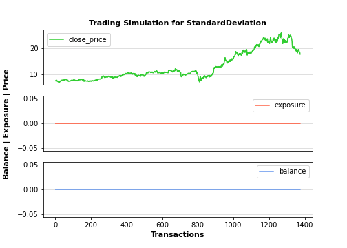
It is clear that the zero SD simulation statistics does not bring any value to our trading strategy.
Let’s look at the Stochastic Momentum Index (SMI) – an indicator of momentum for a security. The SMI is used in technical analysis as a refined alternative to a traditional stochastic oscillator. The SMI is a calculation of the distance of a security’s current closing price as it relates to the median high and low range of prices.
from tti.indicators import StochasticOscillator
stosc_indicator = StochasticOscillator(input_data=df)
Get indicator’s value for a specific date
print(‘\nTechnical Indicator value at 2014-01-07:’, stosc_indicator.getTiValue(‘2014-01-07’))
Get the most recent indicator’s value
print(‘\nMost recent Technical Indicator value:’, stosc_indicator.getTiValue())
Get signal foom indicator
print(‘\nTechnical Indicator signal:’, stosc_indicator.getTiSignal())
Show the Graph for the calculated Technical Indicator
stosc_indicator.getTiGraph().show()
Save the Graph for the calculated Technical Indicator
stosc_indicator.getTiGraph().savefig(‘../TTI/example_stosc.png’)
print(‘\nGraph for the calculated fo indicator data, saved.’)
Execute simulation based on trading signals
simulation_data, simulation_statistics, simulation_graph = \
stosc_indicator.getTiSimulation(
close_values=df[[‘close’]], max_exposure=None,
short_exposure_factor=1.5)
print(‘\nSimulation Data:\n’, simulation_data)
print(‘\nSimulation Statistics:\n’, simulation_statistics)
Save the Graph for the executed trading signal simulation
simulation_graph.savefig(‘../TTI/simulation_stosc.png’)
print(‘\nGraph for the executed trading signal simulation, saved.’)
from tti.indicators import StochasticOscillator
stosc_indicator = StochasticOscillator(input_data=df)
Get indicator’s value for a specific date
print(‘\nTechnical Indicator value at 2022-06-15:’, stosc_indicator.getTiValue(‘2022-06-15’))
Get the most recent indicator’s value
print(‘\nMost recent Technical Indicator value:’, stosc_indicator.getTiValue())
Get signal from indicator
print(‘\nTechnical Indicator signal:’, stosc_indicator.getTiSignal())
Show the Graph for the calculated Technical Indicator
stosc_indicator.getTiGraph().show()
Save the Graph for the calculated Technical Indicator
stosc_indicator.getTiGraph().savefig(‘../TTI/example_stosc.png’)
print(‘\nGraph for the calculated fo indicator data, saved.’)
Execute simulation based on trading signals
simulation_data, simulation_statistics, simulation_graph = \
stosc_indicator.getTiSimulation(
close_values=df[[‘close’]], max_exposure=None,
short_exposure_factor=1.5)
print(‘\nSimulation Data:\n’, simulation_data)
print(‘\nSimulation Statistics:\n’, simulation_statistics)
Save the Graph for the executed trading signal simulation
simulation_graph.savefig(‘../TTI/simulation_stosc.png’)
print(‘\nGraph for the executed trading signal simulation, saved.’)
Technical Indicator value at 2022-06-15: [28.1915, 19.5035]

Most recent Technical Indicator value: [3.4314, 19.0516]

Technical Indicator signal: ('hold', 0)

Graph for the calculated fo indicator data, saved.

Simulation Data:
            signal open_trading_action stock_value    exposure portfolio_value  \
Date
2017-01-03   hold                none        7.37         0.0             0.0
2017-01-04   hold                none       7.565         0.0             0.0
2017-01-05   hold                none        7.51         0.0             0.0
2017-01-06   hold                none        7.41         0.0             0.0
2017-01-09   hold                none        7.48         0.0             0.0
...           ...                 ...         ...         ...             ...
2022-06-10   hold                none       18.33  371.910004     -164.969999
2022-06-13   hold                none       17.85  371.910004     -160.650003
2022-06-14    buy                long       18.24  390.150003     -145.919998
2022-06-15   hold                none   18.290001  371.910004     -164.610008
2022-06-16   hold                none       17.67  371.910004     -159.030001

             earnings     balance
Date
2017-01-03        0.0         0.0
2017-01-04        0.0         0.0
2017-01-05        0.0         0.0
2017-01-06        0.0         0.0
2017-01-09        0.0         0.0
...               ...         ...
2022-06-10  60.840003 -104.129996
2022-06-13  60.840003      -99.81
2022-06-14  60.840003  -85.079995
2022-06-15  60.890005 -103.720004
2022-06-16  60.890005  -98.139996

[1374 rows x 7 columns]

Simulation Statistics:
 {'number_of_trading_days': 1374, 'number_of_buy_signals': 146, 'number_of_ignored_buy_signals': 0, 'number_of_sell_signals': 257, 'number_of_ignored_sell_signals': 0, 'last_stock_value': 17.67, 'last_exposure': 371.91, 'last_open_long_positions': 5, 'last_open_short_positions': 14, 'last_portfolio_value': -159.03, 'last_earnings': 60.89, 'final_balance': -98.14}

Graph for the executed trading signal simulation, saved.
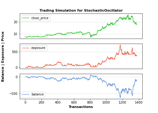
Let’s plot the Swing Index (SI) – a technical indicator that attempts to predict future short-term price action. The Swing Index advertises itself as a tool for very short-term trading.
from tti.indicators import SwingIndex
swind_indicator = SwingIndex(input_data=df)
Get indicator’s value for a specific date
print(‘\nTechnical Indicator value at 2022-06-15:’, swind_indicator.getTiValue(‘2022-06-15’))
Get the most recent indicator’s value
print(‘\nMost recent Technical Indicator value:’, swind_indicator.getTiValue())
Get signal from indicator
print(‘\nTechnical Indicator signal:’, swind_indicator.getTiSignal())
Show the Graph for the calculated Technical Indicator
swind_indicator.getTiGraph().show()
Save the Graph for the calculated Technical Indicator
swind_indicator.getTiGraph().savefig(‘../TTI/example_swind.png’)
print(‘\nGraph for the calculated fo indicator data, saved.’)
Execute simulation based on trading signals
simulation_data, simulation_statistics, simulation_graph = \
swind_indicator.getTiSimulation(
close_values=df[[‘close’]], max_exposure=None,
short_exposure_factor=1.5)
print(‘\nSimulation Data:\n’, simulation_data)
print(‘\nSimulation Statistics:\n’, simulation_statistics)
Save the Graph for the executed trading signal simulation
simulation_graph.savefig(‘../TTI/simulation_swind.png’)
print(‘\nGraph for the executed trading signal simulation, saved.’)
Technical Indicator value at 2022-06-15: [2.5863]

Most recent Technical Indicator value: [-9.3462]

Technical Indicator signal: ('buy', -1)
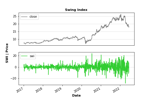
Graph for the calculated fo indicator data, saved.

Simulation Data:
            signal open_trading_action stock_value    exposure portfolio_value  \
Date
2017-01-03   hold                none        7.37         0.0             0.0
2017-01-04   hold                none       7.565         0.0             0.0
2017-01-05    buy                long        7.51        7.51            7.51
2017-01-06   hold                none        7.41        7.51            7.41
2017-01-09   sell               short        7.48       18.73             0.0
...           ...                 ...         ...         ...             ...
2022-06-10   hold                none       18.33     353.695         -109.98
2022-06-13   hold                none       17.85     353.695     -107.100002
2022-06-14   sell               short       18.24  381.054999     -127.679998
2022-06-15   hold                none   18.290001  381.054999     -128.030006
2022-06-16    buy                long       17.67     371.365          -88.35

             earnings    balance
Date
2017-01-03        0.0        0.0
2017-01-04        0.0        0.0
2017-01-05        0.0       7.51
2017-01-06        0.0       7.41
2017-01-09        0.0        0.0
...               ...        ...
2022-06-10  98.639989  -11.34001
2022-06-13  98.639989  -8.460013
2022-06-14  98.639989 -29.040009
2022-06-15  98.639989 -29.390017
2022-06-16  99.209989  10.859989

[1374 rows x 7 columns]

Simulation Statistics:
 {'number_of_trading_days': 1374, 'number_of_buy_signals': 322, 'number_of_ignored_buy_signals': 0, 'number_of_sell_signals': 320, 'number_of_ignored_sell_signals': 0, 'last_stock_value': 17.67, 'last_exposure': 371.36, 'last_open_long_positions': 7, 'last_open_short_positions': 12, 'last_portfolio_value': -88.35, 'last_earnings': 99.21, 'final_balance': 10.86}

Graph for the executed trading signal simulation, saved.
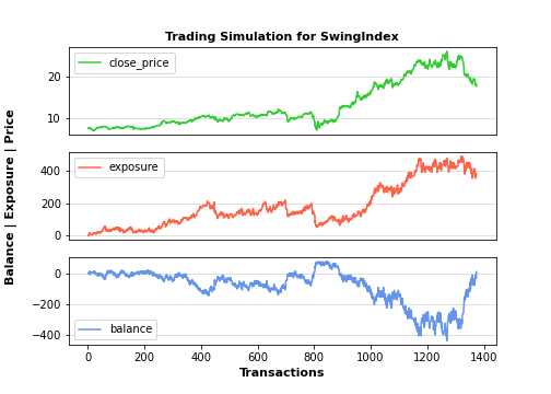
Let’s look at the Time Series Forecast indicator (TSF) that shows the statistical trend of a security’s price over a specified time period. This indicator is referred to as a moving linear regression that is similar to a moving average. The Time Series Forecast (TSF) indicator is based upon a regression-based forecast model.
from tti.indicators import TimeSeriesForecast
tsf_indicator = TimeSeriesForecast(input_data=df)
Get indicator’s value for a specific date
print(‘\nTechnical Indicator value at 2022-06-15:’, tsf_indicator.getTiValue(‘2022-06-15’))
Get the most recent indicator’s value
print(‘\nMost recent Technical Indicator value:’, tsf_indicator.getTiValue())
Get signal from indicator
print(‘\nTechnical Indicator signal:’, tsf_indicator.getTiSignal())
Show the Graph for the calculated Technical Indicator
tsf_indicator.getTiGraph().show()
Save the Graph for the calculated Technical Indicator
tsf_indicator.getTiGraph().savefig(‘../TTI/example_tsf.png’)
print(‘\nGraph for the calculated fo indicator data, saved.’)
Execute simulation based on trading signals
simulation_data, simulation_statistics, simulation_graph = \
tsf_indicator.getTiSimulation(
close_values=df[[‘close’]], max_exposure=None,
short_exposure_factor=1.5)
print(‘\nSimulation Data:\n’, simulation_data)
print(‘\nSimulation Statistics:\n’, simulation_statistics)
Save the Graph for the executed trading signal simulation
simulation_graph.savefig(‘../TTI/simulation_tsf.png’)
print(‘\nGraph for the executed trading signal simulation, saved.’)
Technical Indicator value at 2022-06-15: [18.3758]

Most recent Technical Indicator value: [17.972]

Technical Indicator signal: ('hold', 0)

Graph for the calculated fo indicator data, saved.

Simulation Data:
            signal open_trading_action stock_value    exposure portfolio_value  \
Date
2017-01-03   hold                none        7.37         0.0             0.0
2017-01-04   hold                none       7.565         0.0             0.0
2017-01-05   hold                none        7.51         0.0             0.0
2017-01-06   hold                none        7.41         0.0             0.0
2017-01-09   hold                none        7.48         0.0             0.0
...           ...                 ...         ...         ...             ...
2022-06-10   hold                none       18.33  120.789999             0.0
2022-06-13   hold                none       17.85  120.789999             0.0
2022-06-14   hold                none       18.24  120.789999             0.0
2022-06-15   hold                none   18.290001  120.789999             0.0
2022-06-16   hold                none       17.67  120.789999             0.0

             earnings    balance
Date
2017-01-03        0.0        0.0
2017-01-04        0.0        0.0
2017-01-05        0.0        0.0
2017-01-06        0.0        0.0
2017-01-09        0.0        0.0
...               ...        ...
2022-06-10  54.430006  54.430006
2022-06-13  54.430006  54.430006
2022-06-14  54.430006  54.430006
2022-06-15  54.430006  54.430006
2022-06-16  54.430006  54.430006

[1374 rows x 7 columns]

Simulation Statistics:
 {'number_of_trading_days': 1374, 'number_of_buy_signals': 156, 'number_of_ignored_buy_signals': 0, 'number_of_sell_signals': 156, 'number_of_ignored_sell_signals': 0, 'last_stock_value': 17.67, 'last_exposure': 120.79, 'last_open_long_positions': 3, 'last_open_short_positions': 3, 'last_portfolio_value': 0.0, 'last_earnings': 54.43, 'final_balance': 54.43}

Graph for the executed trading signal simulation, saved.

Let’s look at the triple exponential moving average (TEMA) that uses multiple EMA calculations and subtracts out the lag to create a trend following indicator that reacts quickly to price changes. The TEMA can help identify trend direction, signal potential short-term trend changes or pullbacks, and provide support or resistance.
from tti.indicators import TripleExponentialMovingAverage
tema_indicator = TripleExponentialMovingAverage(input_data=df)
Get indicator’s value for a specific date
print(‘\nTechnical Indicator value at 2022-06-15:’, tema_indicator.getTiValue(‘2022-06-15’))
Get the most recent indicator’s value
print(‘\nMost recent Technical Indicator value:’, tema_indicator.getTiValue())
Get signal from indicator
print(‘\nTechnical Indicator signal:’, tema_indicator.getTiSignal())
Show the Graph for the calculated Technical Indicator
tema_indicator.getTiGraph().show()
Save the Graph for the calculated Technical Indicator
tema_indicator.getTiGraph().savefig(‘../TTI/example_tema.png’)
print(‘\nGraph for the calculated fo indicator data, saved.’)
Execute simulation based on trading signals
simulation_data, simulation_statistics, simulation_graph = \
tema_indicator.getTiSimulation(
close_values=df[[‘close’]], max_exposure=None,
short_exposure_factor=1.5)
print(‘\nSimulation Data:\n’, simulation_data)
print(‘\nSimulation Statistics:\n’, simulation_statistics)
Save the Graph for the executed trading signal simulation
simulation_graph.savefig(‘../TTI/simulation_tema.png’)
print(‘\nGraph for the executed trading signal simulation, saved.’)
Technical Indicator value at 2022-06-15: [18.1228]

Most recent Technical Indicator value: [17.7593]

Technical Indicator signal: ('buy', -1)
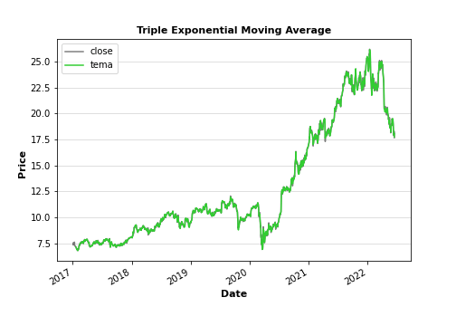
Graph for the calculated fo indicator data, saved.

Simulation Data:
            signal open_trading_action stock_value    exposure portfolio_value  \
Date
2017-01-03   hold                none        7.37         0.0             0.0
2017-01-04   hold                none       7.565         0.0             0.0
2017-01-05   hold                none        7.51         0.0             0.0
2017-01-06   hold                none        7.41         0.0             0.0
2017-01-09   hold                none        7.48         0.0             0.0
...           ...                 ...         ...         ...             ...
2022-06-10    buy                long       18.33  761.887493     -146.639999
2022-06-13    buy                long       17.85  752.917495     -107.100002
2022-06-14   sell               short       18.24  762.427494     -145.919998
2022-06-15   sell               short   18.290001  789.862495     -164.610008
2022-06-16    buy                long       17.67  752.737494         -106.02

              earnings     balance
Date
2017-01-03         0.0         0.0
2017-01-04         0.0         0.0
2017-01-05         0.0         0.0
2017-01-06         0.0         0.0
2017-01-09         0.0         0.0
...                ...         ...
2022-06-10   211.43999    64.79999
2022-06-13  211.469988  104.369986
2022-06-14  211.859988    65.93999
2022-06-15  211.859988   47.249979
2022-06-16  213.049988  107.029988

[1374 rows x 7 columns]

Simulation Statistics:
 {'number_of_trading_days': 1374, 'number_of_buy_signals': 665, 'number_of_ignored_buy_signals': 0, 'number_of_sell_signals': 697, 'number_of_ignored_sell_signals': 0, 'last_stock_value': 17.67, 'last_exposure': 752.74, 'last_open_long_positions': 17, 'last_open_short_positions': 23, 'last_portfolio_value': -106.02, 'last_earnings': 213.05, 'final_balance': 107.03}

Graph for the executed trading signal simulation, saved.

let’s consider the Typical Price indicator that provides a simple, single-line plot of the day’s average price. Some investors use the Typical Price rather than the closing price when creating moving-average penetration systems. The Typical Price is a building block of the Money Flow Index.
from tti.indicators import TypicalPrice
typ_indicator = TypicalPrice(input_data=df)
Get indicator’s value for a specific date
print(‘\nTechnical Indicator value at 2022-06-15:’, typ_indicator.getTiValue(‘2022-06-15’))
Get the most recent indicator’s value
print(‘\nMost recent Technical Indicator value:’, typ_indicator.getTiValue())
Get signal from indicator
print(‘\nTechnical Indicator signal:’, typ_indicator.getTiSignal())
Show the Graph for the calculated Technical Indicator
typ_indicator.getTiGraph().show()
Save the Graph for the calculated Technical Indicator
typ_indicator.getTiGraph().savefig(‘../TTI/example_typ.png’)
print(‘\nGraph for the calculated fo indicator data, saved.’)
Execute simulation based on trading signals
simulation_data, simulation_statistics, simulation_graph = \
typ_indicator.getTiSimulation(
close_values=df[[‘close’]], max_exposure=None,
short_exposure_factor=1.5)
print(‘\nSimulation Data:\n’, simulation_data)
print(‘\nSimulation Statistics:\n’, simulation_statistics)
Save the Graph for the executed trading signal simulation
simulation_graph.savefig(‘../TTI/simulation_typ.png’)
print(‘\nGraph for the executed trading signal simulation, saved.’)
Technical Indicator value at 2022-06-15: [18.1733]

Most recent Technical Indicator value: [17.6867]

Technical Indicator signal: ('hold', 0)

Graph for the calculated fo indicator data, saved.

Simulation Data:
            signal open_trading_action stock_value exposure portfolio_value  \
Date
2017-01-03   hold                none        7.37      0.0             0.0
2017-01-04   hold                none       7.565      0.0             0.0
2017-01-05   hold                none        7.51      0.0             0.0
2017-01-06   hold                none        7.41      0.0             0.0
2017-01-09   hold                none        7.48      0.0             0.0
...           ...                 ...         ...      ...             ...
2022-06-10   hold                none       18.33    272.4      201.629999
2022-06-13   hold                none       17.85    272.4      196.350004
2022-06-14   hold                none       18.24    272.4      200.639997
2022-06-15   hold                none   18.290001    272.4       201.19001
2022-06-16   hold                none       17.67    272.4      194.370001

              earnings     balance
Date
2017-01-03         0.0         0.0
2017-01-04         0.0         0.0
2017-01-05         0.0         0.0
2017-01-06         0.0         0.0
2017-01-09         0.0         0.0
...                ...         ...
2022-06-10  149.179998  350.809998
2022-06-13  149.179998  345.530003
2022-06-14  149.179998  349.819996
2022-06-15  149.179998  350.370008
2022-06-16  149.179998  343.549999

[1374 rows x 7 columns]

Simulation Statistics:
 {'number_of_trading_days': 1374, 'number_of_buy_signals': 898, 'number_of_ignored_buy_signals': 0, 'number_of_sell_signals': 0, 'number_of_ignored_sell_signals': 0, 'last_stock_value': 17.67, 'last_exposure': 272.4, 'last_open_long_positions': 11, 'last_open_short_positions': 0, 'last_portfolio_value': 194.37, 'last_earnings': 149.18, 'final_balance': 343.55}

Graph for the executed trading signal simulation, saved.

Let’s plot the Ultimate Oscillator indicator (UO) – a technical analysis tool used to measure momentum across three varying time frames. The problem with many momentum oscillators is that after a rapid advance or decline in price, they can form false divergence trading signals. For example, after a rapid rise in price, a bearish divergence signal may present itself, however the price continues to rise. The UO attempts to correct this by using multiple time frames in its calculation as opposed to just one time frame which is what is used in most other momentum oscillators.
from tti.indicators import UltimateOscillator
uosc_indicator = UltimateOscillator(input_data=df)
Get indicator’s value for a specific date
print(‘\nTechnical Indicator value at 2022-06-15:’, uosc_indicator.getTiValue(‘2022-06-15’))
Get the most recent indicator’s value
print(‘\nMost recent Technical Indicator value:’, uosc_indicator.getTiValue())
Get signal from indicator
print(‘\nTechnical Indicator signal:’, uosc_indicator.getTiSignal())
Show the Graph for the calculated Technical Indicator
uosc_indicator.getTiGraph().show()
Save the Graph for the calculated Technical Indicator
uosc_indicator.getTiGraph().savefig(‘../TTI/example_uosc.png’)
print(‘\nGraph for the calculated fo indicator data, saved.’)
Execute simulation based on trading signals
simulation_data, simulation_statistics, simulation_graph = \
uosc_indicator.getTiSimulation(
close_values=df[[‘close’]], max_exposure=None,
short_exposure_factor=1.5)
print(‘\nSimulation Data:\n’, simulation_data)
print(‘\nSimulation Statistics:\n’, simulation_statistics)
Save the Graph for the executed trading signal simulation
simulation_graph.savefig(‘../TTI/simulation_uosc.png’)
print(‘\nGraph for the executed trading signal simulation, saved.’)
Technical Indicator value at 2022-06-15: [46.258]

Most recent Technical Indicator value: [37.8327]

Technical Indicator signal: ('buy', -1)

Graph for the calculated fo indicator data, saved.

Simulation Data:
            signal open_trading_action stock_value    exposure portfolio_value  \
Date
2017-01-03   hold                none        7.37         0.0             0.0
2017-01-04   hold                none       7.565         0.0             0.0
2017-01-05   hold                none        7.51         0.0             0.0
2017-01-06   hold                none        7.41         0.0             0.0
2017-01-09   hold                none        7.48         0.0             0.0
...           ...                 ...         ...         ...             ...
2022-06-10    buy                long       18.33  573.349998      476.579998
2022-06-13   hold                none       17.85  573.349998       464.10001
2022-06-14   hold                none       18.24  573.349998      474.239994
2022-06-15   hold                none   18.290001  573.349998      475.540024
2022-06-16    buy                long       17.67  591.019999      477.090002

              earnings     balance
Date
2017-01-03         0.0         0.0
2017-01-04         0.0         0.0
2017-01-05         0.0         0.0
2017-01-06         0.0         0.0
2017-01-09         0.0         0.0
...                ...         ...
2022-06-10  159.384996  635.964994
2022-06-13  159.384996  623.485006
2022-06-14  159.384996   633.62499
2022-06-15  159.384996   634.92502
2022-06-16  159.384996  636.474998

[1374 rows x 7 columns]

Simulation Statistics:
 {'number_of_trading_days': 1374, 'number_of_buy_signals': 1098, 'number_of_ignored_buy_signals': 0, 'number_of_sell_signals': 0, 'number_of_ignored_sell_signals': 0, 'last_stock_value': 17.67, 'last_exposure': 591.02, 'last_open_long_positions': 27, 'last_open_short_positions': 0, 'last_portfolio_value': 477.09, 'last_earnings': 159.38, 'final_balance': 636.47}

Graph for the executed trading signal simulation, saved.
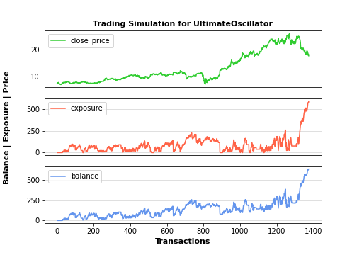
Let’s calculate the Vertical Horizontal Filter (VHF) that determines whether prices are in a trending phase or a congestion phase.
from tti.indicators import VerticalHorizontalFilter
vhf_indicator = VerticalHorizontalFilter(input_data=df)
Get indicator’s value for a specific date
print(‘\nTechnical Indicator value at 2022-06-15:’, vhf_indicator.getTiValue(‘2022-06-15’))
Get the most recent indicator’s value
print(‘\nMost recent Technical Indicator value:’, vhf_indicator.getTiValue())
Get signal from indicator
print(‘\nTechnical Indicator signal:’, vhf_indicator.getTiSignal())
Show the Graph for the calculated Technical Indicator
vhf_indicator.getTiGraph().show()
Save the Graph for the calculated Technical Indicator
vhf_indicator.getTiGraph().savefig(‘../TTI/example_vhf.png’)
print(‘\nGraph for the calculated fo indicator data, saved.’)
Execute simulation based on trading signals
simulation_data, simulation_statistics, simulation_graph = \
vhf_indicator.getTiSimulation(
close_values=df[[‘close’]], max_exposure=None,
short_exposure_factor=1.5)
print(‘\nSimulation Data:\n’, simulation_data)
print(‘\nSimulation Statistics:\n’, simulation_statistics)
Save the Graph for the executed trading signal simulation
simulation_graph.savefig(‘../TTI/simulation_vhf.png’)
print(‘\nGraph for the executed trading signal simulation, saved.’)
Technical Indicator value at 2022-06-15: [0.5886]

Most recent Technical Indicator value: [0.3158]

Technical Indicator signal: ('hold', 0)
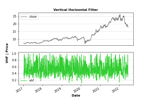
Graph for the calculated fo indicator data, saved.

Simulation Data:
            signal open_trading_action stock_value exposure portfolio_value  \
Date
2017-01-03   hold                none        7.37      0.0             0.0
2017-01-04   hold                none       7.565      0.0             0.0
2017-01-05   hold                none        7.51      0.0             0.0
2017-01-06   hold                none        7.41      0.0             0.0
2017-01-09   hold                none        7.48      0.0             0.0
...           ...                 ...         ...      ...             ...
2022-06-10    buy                long       18.33   127.24          109.98
2022-06-13    buy                long       17.85   145.09      124.950003
2022-06-14   hold                none       18.24   127.24      109.439999
2022-06-15   hold                none   18.290001   127.24      109.740005
2022-06-16   hold                none       17.67   127.24          106.02

             earnings     balance
Date
2017-01-03        0.0         0.0
2017-01-04        0.0         0.0
2017-01-05        0.0         0.0
2017-01-06        0.0         0.0
2017-01-09        0.0         0.0
...               ...         ...
2022-06-10  33.454995  143.434995
2022-06-13  33.454995  158.404998
2022-06-14  33.844995  143.284993
2022-06-15  33.844995     143.585
2022-06-16  33.844995  139.864995

[1374 rows x 7 columns]

Simulation Statistics:
 {'number_of_trading_days': 1374, 'number_of_buy_signals': 168, 'number_of_ignored_buy_signals': 0, 'number_of_sell_signals': 27, 'number_of_ignored_sell_signals': 0, 'last_stock_value': 17.67, 'last_exposure': 127.24, 'last_open_long_positions': 6, 'last_open_short_positions': 0, 'last_portfolio_value': 106.02, 'last_earnings': 33.84, 'final_balance': 139.86}

Graph for the executed trading signal simulation, saved.
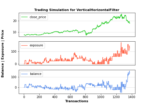
Another indicator is the Chaikin Volatility Indicator. It is the difference between two moving averages of a volume weighted accumulation-distribution line. By comparing the spread between a security’s high and low prices, it quantifies volatility as a widening of the range between the high and the low price.
One interpretation of these calculations assumes that market tops are frequently accompanied by increased volatility (as investors get nervous and become indecisive) and latter stages of a market bottom are generally accompanied by decreased volatility. Chaikin has written that an increase in the Volatility Indicator over a relatively short time period indicates that a bottom is near and that a decrease in volatility over a longer time period indicates an approaching top.
Marc Chaikin measures volatility as the trading range between high and low for each period. This does not take trading gaps into account as Average True Range does.
Chaikin Volatility should be used in conjunction with a moving average system or price envelopes.
from tti.indicators import VolatilityChaikins
volc_indicator = VolatilityChaikins(input_data=df)
Get indicator’s value for a specific date
print(‘\nTechnical Indicator value at 2022-06-15:’, volc_indicator.getTiValue(‘2022-06-15’))
Get the most recent indicator’s value
print(‘\nMost recent Technical Indicator value:’, volc_indicator.getTiValue())
Get signal from indicator
print(‘\nTechnical Indicator signal:’, volc_indicator.getTiSignal())
Show the Graph for the calculated Technical Indicator
volc_indicator.getTiGraph().show()
Save the Graph for the calculated Technical Indicator
volc_indicator.getTiGraph().savefig(‘../TTI/example_volc.png’)
print(‘\nGraph for the calculated fo indicator data, saved.’)
Execute simulation based on trading signals
simulation_data, simulation_statistics, simulation_graph = \
volc_indicator.getTiSimulation(
close_values=df[[‘close’]], max_exposure=None,
short_exposure_factor=1.5)
print(‘\nSimulation Data:\n’, simulation_data)
print(‘\nSimulation Statistics:\n’, simulation_statistics)
Save the Graph for the executed trading signal simulation
simulation_graph.savefig(‘../TTI/simulation_volc.png’)
print(‘\nGraph for the executed trading signal simulation, saved.’)
Technical Indicator value at 2022-06-15: [-9.5633]

Most recent Technical Indicator value: [-12.3036]

Technical Indicator signal: ('hold', 0)

Graph for the calculated fo indicator data, saved.

Simulation Data:
            signal open_trading_action stock_value  exposure portfolio_value  \
Date
2017-01-03   hold                none        7.37       0.0             0.0
2017-01-04   hold                none       7.565       0.0             0.0
2017-01-05   hold                none        7.51       0.0             0.0
2017-01-06   hold                none        7.41       0.0             0.0
2017-01-09   hold                none        7.48       0.0             0.0
...           ...                 ...         ...       ...             ...
2022-06-10    buy                long       18.33  631.8375     -201.629999
2022-06-13    buy                long       17.85  649.6875     -178.500004
2022-06-14   hold                none       18.24  631.8375     -200.639997
2022-06-15   hold                none   18.290001  631.8375      -201.19001
2022-06-16   hold                none       17.67  631.8375     -194.370001

              earnings    balance
Date
2017-01-03         0.0        0.0
2017-01-04         0.0        0.0
2017-01-05         0.0        0.0
2017-01-06         0.0        0.0
2017-01-09         0.0        0.0
...                ...        ...
2022-06-10  106.205001 -95.424998
2022-06-13  106.205001 -72.295002
2022-06-14  106.595001 -94.044997
2022-06-15  106.595001 -94.595009
2022-06-16  106.595001    -87.775

[1374 rows x 7 columns]

Simulation Statistics:
 {'number_of_trading_days': 1374, 'number_of_buy_signals': 368, 'number_of_ignored_buy_signals': 0, 'number_of_sell_signals': 368, 'number_of_ignored_sell_signals': 0, 'last_stock_value': 17.67, 'last_exposure': 631.84, 'last_open_long_positions': 11, 'last_open_short_positions': 22, 'last_portfolio_value': -194.37, 'last_earnings': 106.6, 'final_balance': -87.78}

Graph for the executed trading signal simulation, saved.
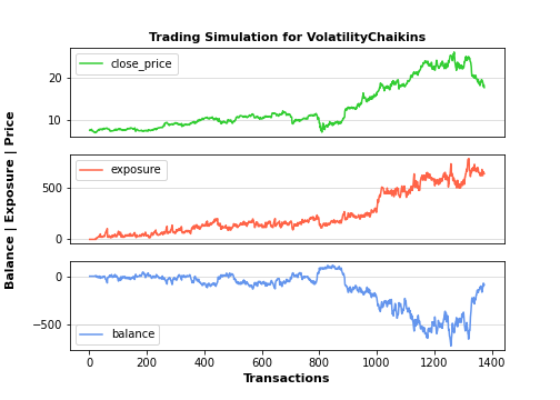
Let’s look at the Volume Oscillator (VO). The VO works on the technical premise that it is not the actual level of volume, but the change in volume relative to the recent past that has more technical significance. The VO displays the difference between two moving averages of a security’s volume expressed as a percentage.
from tti.indicators import VolumeOscillator
volumeosc_indicator = VolumeOscillator(input_data=df)
Get indicator’s value for a specific date
print(‘\nTechnical Indicator value at 2022-06-15:’, volumeosc_indicator.getTiValue(‘2022-06-15’))
Get the most recent indicator’s value
print(‘\nMost recent Technical Indicator value:’, volumeosc_indicator.getTiValue())
Get signal from indicator
print(‘\nTechnical Indicator signal:’, volumeosc_indicator.getTiSignal())
Show the Graph for the calculated Technical Indicator
volumeosc_indicator.getTiGraph().show()
Save the Graph for the calculated Technical Indicator
volumeosc_indicator.getTiGraph().savefig(‘../TTI/example_volumeosc.png’)
print(‘\nGraph for the calculated fo indicator data, saved.’)
Execute simulation based on trading signals
simulation_data, simulation_statistics, simulation_graph = \
volumeosc_indicator.getTiSimulation(
close_values=df[[‘close’]], max_exposure=None,
short_exposure_factor=1.5)
print(‘\nSimulation Data:\n’, simulation_data)
print(‘\nSimulation Statistics:\n’, simulation_statistics)
Save the Graph for the executed trading signal simulation
simulation_graph.savefig(‘../TTI/simulation_volumeosc.png’)
print(‘\nGraph for the executed trading signal simulation, saved.’)
Technical Indicator value at 2022-06-15: [3575320.0]

Most recent Technical Indicator value: [726180.0]

Technical Indicator signal: ('hold', 0)

Graph for the calculated fo indicator data, saved.

Simulation Data:
            signal open_trading_action stock_value   exposure portfolio_value  \
Date
2017-01-03   hold                none        7.37        0.0             0.0
2017-01-04   hold                none       7.565        0.0             0.0
2017-01-05   hold                none        7.51        0.0             0.0
2017-01-06   hold                none        7.41        0.0             0.0
2017-01-09   hold                none        7.48        0.0             0.0
...           ...                 ...         ...        ...             ...
2022-06-10   hold                none       18.33  39.094999             0.0
2022-06-13   hold                none       17.85  39.094999             0.0
2022-06-14    buy                long       18.24  57.334999           18.24
2022-06-15    buy                long   18.290001     57.385       18.290001
2022-06-16   hold                none       17.67     57.385           17.67

             earnings    balance
Date
2017-01-03        0.0        0.0
2017-01-04        0.0        0.0
2017-01-05        0.0        0.0
2017-01-06        0.0        0.0
2017-01-09        0.0        0.0
...               ...        ...
2022-06-10  18.950006  18.950006
2022-06-13  18.950006  18.950006
2022-06-14  18.950006  37.190006
2022-06-15  19.000007  37.290008
2022-06-16  19.000007  36.670007

[1374 rows x 7 columns]

Simulation Statistics:
 {'number_of_trading_days': 1374, 'number_of_buy_signals': 77, 'number_of_ignored_buy_signals': 0, 'number_of_sell_signals': 29, 'number_of_ignored_sell_signals': 0, 'last_stock_value': 17.67, 'last_exposure': 57.39, 'last_open_long_positions': 2, 'last_open_short_positions': 1, 'last_portfolio_value': 17.67, 'last_earnings': 19.0, 'final_balance': 36.67}

Graph for the executed trading signal simulation, saved.

Let’s plot the volume rate of change. This is the indicator that shows whether or not a volume trend is developing in either an up or down direction.
from tti.indicators import VolumeRateOfChange
vroc_indicator = VolumeRateOfChange(input_data=df)
Get indicator’s value for a specific date
print(‘\nTechnical Indicator value at 2022-06-15:’, vroc_indicator.getTiValue(‘2022-06-15’))
Get the most recent indicator’s value
print(‘\nMost recent Technical Indicator value:’, vroc_indicator.getTiValue())
Get signal from indicator
print(‘\nTechnical Indicator signal:’, vroc_indicator.getTiSignal())
Show the Graph for the calculated Technical Indicator
vroc_indicator.getTiGraph().show()
Save the Graph for the calculated Technical Indicator
vroc_indicator.getTiGraph().savefig(‘../TTI/example_vroc.png’)
print(‘\nGraph for the calculated fo indicator data, saved.’)
Execute simulation based on trading signals
simulation_data, simulation_statistics, simulation_graph = \
vroc_indicator.getTiSimulation(
close_values=df[[‘close’]], max_exposure=None,
short_exposure_factor=1.5)
print(‘\nSimulation Data:\n’, simulation_data)
print(‘\nSimulation Statistics:\n’, simulation_statistics)
Save the Graph for the executed trading signal simulation
simulation_graph.savefig(‘../TTI/simulation_vroc.png’)
print(‘\nGraph for the executed trading signal simulation, saved.’)
Technical Indicator value at 2022-06-15: [418.1639]

Most recent Technical Indicator value: [-2.4806]

Technical Indicator signal: ('hold', 0)
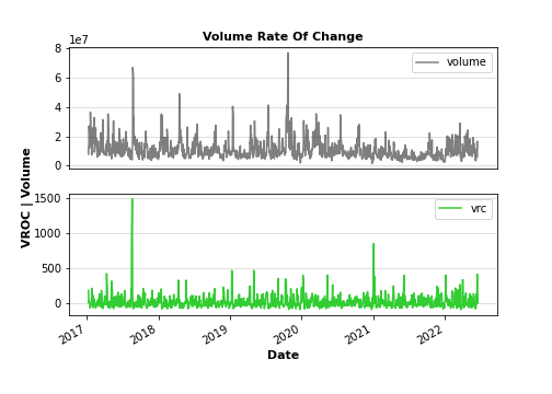
Graph for the calculated fo indicator data, saved.

Simulation Data:
            signal open_trading_action stock_value    exposure portfolio_value  \
Date
2017-01-03   hold                none        7.37         0.0             0.0
2017-01-04   hold                none       7.565         0.0             0.0
2017-01-05   hold                none        7.51         0.0             0.0
2017-01-06   hold                none        7.41         0.0             0.0
2017-01-09   hold                none        7.48         0.0             0.0
...           ...                 ...         ...         ...             ...
2022-06-10   sell               short       18.33      366.16          -91.65
2022-06-13   sell               short       17.85  338.230002      -71.400002
2022-06-14   hold                none       18.24  338.230002      -72.959999
2022-06-15   hold                none   18.290001  338.230002      -73.160004
2022-06-16   hold                none       17.67  311.455001          -53.01

             earnings    balance
Date
2017-01-03        0.0        0.0
2017-01-04        0.0        0.0
2017-01-05        0.0        0.0
2017-01-06        0.0        0.0
2017-01-09        0.0        0.0
...               ...        ...
2022-06-10     87.365  -4.284999
2022-06-13  88.134999  16.734997
2022-06-14  88.134999     15.175
2022-06-15  88.134999  14.974995
2022-06-16  88.314999  35.304999

[1374 rows x 7 columns]

Simulation Statistics:
 {'number_of_trading_days': 1374, 'number_of_buy_signals': 269, 'number_of_ignored_buy_signals': 0, 'number_of_sell_signals': 294, 'number_of_ignored_sell_signals': 0, 'last_stock_value': 17.67, 'last_exposure': 311.46, 'last_open_long_positions': 6, 'last_open_short_positions': 9, 'last_portfolio_value': -53.01, 'last_earnings': 88.31, 'final_balance': 35.3}

Graph for the executed trading signal simulation, saved.

Next, we plot the Weighted Close indicator as the average of High, Low and doubled Closing price. As the same as in style to Typical Price, Weighted Close is the technical indicator that measures the mean change in a security’s price. Weighted Closed indicator’s main purpose is to filter the Moving Average System.
from tti.indicators import WeightedClose
wc_indicator = WeightedClose(input_data=df)
Get indicator’s value for a specific date
print(‘\nTechnical Indicator value at 2022-06-15:’, wc_indicator.getTiValue(‘2022-06-15’))
Get the most recent indicator’s value
print(‘\nMost recent Technical Indicator value:’, wc_indicator.getTiValue())
Get signal from indicator
print(‘\nTechnical Indicator signal:’, wc_indicator.getTiSignal())
Show the Graph for the calculated Technical Indicator
wc_indicator.getTiGraph().show()
Save the Graph for the calculated Technical Indicator
wc_indicator.getTiGraph().savefig(‘../TTI/example_wc.png’)
print(‘\nGraph for the calculated fo indicator data, saved.’)
Execute simulation based on trading signals
simulation_data, simulation_statistics, simulation_graph = \
wc_indicator.getTiSimulation(
close_values=df[[‘close’]], max_exposure=None,
short_exposure_factor=1.5)
print(‘\nSimulation Data:\n’, simulation_data)
print(‘\nSimulation Statistics:\n’, simulation_statistics)
Save the Graph for the executed trading signal simulation
simulation_graph.savefig(‘../TTI/simulation_wc.png’)
print(‘\nGraph for the executed trading signal simulation, saved.’)
Technical Indicator value at 2022-06-15: [18.2025]

Most recent Technical Indicator value: [17.6825]

Technical Indicator signal: ('buy', -1)
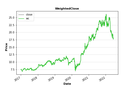
Graph for the calculated fo indicator data, saved.

Simulation Data:
            signal open_trading_action stock_value    exposure portfolio_value  \
Date
2017-01-03   hold                none        7.37         0.0             0.0
2017-01-04   hold                none       7.565         0.0             0.0
2017-01-05    buy                long        7.51        7.51            7.51
2017-01-06   sell               short        7.41      18.625             0.0
2017-01-09   hold                none        7.48      18.625             0.0
...           ...                 ...         ...         ...             ...
2022-06-10   hold                none       18.33  443.789998     -201.629999
2022-06-13   hold                none       17.85  416.579999     -178.500004
2022-06-14   sell               short       18.24  443.939999     -200.639997
2022-06-15   hold                none   18.290001  443.939999      -201.19001
2022-06-16    buy                long       17.67  434.249999     -159.030001

              earnings    balance
Date
2017-01-03         0.0        0.0
2017-01-04         0.0        0.0
2017-01-05         0.0       7.51
2017-01-06         0.0        0.0
2017-01-09         0.0        0.0
...                ...        ...
2022-06-10  102.874992 -98.755007
2022-06-13  103.164991 -75.335013
2022-06-14  103.164991 -97.475007
2022-06-15  103.164991 -98.025019
2022-06-16  103.734991  -55.29501

[1374 rows x 7 columns]

Simulation Statistics:
 {'number_of_trading_days': 1374, 'number_of_buy_signals': 348, 'number_of_ignored_buy_signals': 0, 'number_of_sell_signals': 346, 'number_of_ignored_sell_signals': 0, 'last_stock_value': 17.67, 'last_exposure': 434.25, 'last_open_long_positions': 7, 'last_open_short_positions': 16, 'last_portfolio_value': -159.03, 'last_earnings': 103.73, 'final_balance': -55.3}

Graph for the executed trading signal simulation, saved.

Let’s look at the Wilder’s Smoothing. Also called Wilder’s Smoothed Moving Average, this indicator is similar to the Exponential Moving Average. Compared to other moving averages, Wilders MA responds more slowly to price changes, where an n-period Wilder MA gives similar values to a 2n- period EMA.
from tti.indicators import WildersSmoothing
ws_indicator = WildersSmoothing(input_data=df)
Get indicator’s value for a specific date
print(‘\nTechnical Indicator value at 2022-06-15:’, ws_indicator.getTiValue(‘2022-06-15’))
Get the most recent indicator’s value
print(‘\nMost recent Technical Indicator value:’, ws_indicator.getTiValue())
Get signal from indicator
print(‘\nTechnical Indicator signal:’, ws_indicator.getTiSignal())
Show the Graph for the calculated Technical Indicator
ws_indicator.getTiGraph().show()
Save the Graph for the calculated Technical Indicator
ws_indicator.getTiGraph().savefig(‘../TTI/example_ws.png’)
print(‘\nGraph for the calculated fo indicator data, saved.’)
Execute simulation based on trading signals
simulation_data, simulation_statistics, simulation_graph = \
ws_indicator.getTiSimulation(
close_values=df[[‘close’]], max_exposure=None,
short_exposure_factor=1.5)
print(‘\nSimulation Data:\n’, simulation_data)
print(‘\nSimulation Statistics:\n’, simulation_statistics)
Save the Graph for the executed trading signal simulation
simulation_graph.savefig(‘../TTI/simulation_ws.png’)
print(‘\nGraph for the executed trading signal simulation, saved.’)
Technical Indicator value at 2022-06-15: [18.5693]

Most recent Technical Indicator value: [18.3894]

Technical Indicator signal: ('hold', 0)
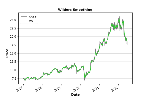
Graph for the calculated fo indicator data, saved.

Simulation Data:
            signal open_trading_action stock_value    exposure portfolio_value  \
Date
2017-01-03   hold                none        7.37         0.0             0.0
2017-01-04   hold                none       7.565         0.0             0.0
2017-01-05   hold                none        7.51         0.0             0.0
2017-01-06   hold                none        7.41         0.0             0.0
2017-01-09   hold                none        7.48         0.0             0.0
...           ...                 ...         ...         ...             ...
2022-06-10   hold                none       18.33  132.579999          -18.33
2022-06-13   hold                none       17.85  132.579999          -17.85
2022-06-14   hold                none       18.24  132.579999          -18.24
2022-06-15   hold                none   18.290001  132.579999      -18.290001
2022-06-16   hold                none       17.67  132.579999          -17.67

             earnings    balance
Date
2017-01-03        0.0        0.0
2017-01-04        0.0        0.0
2017-01-05        0.0        0.0
2017-01-06        0.0        0.0
2017-01-09        0.0        0.0
...               ...        ...
2022-06-10  43.594988  25.264988
2022-06-13  43.594988  25.744987
2022-06-14  43.594988  25.354988
2022-06-15  43.594988  25.304987
2022-06-16  43.594988  25.924988

[1374 rows x 7 columns]

Simulation Statistics:
 {'number_of_trading_days': 1374, 'number_of_buy_signals': 152, 'number_of_ignored_buy_signals': 0, 'number_of_sell_signals': 151, 'number_of_ignored_sell_signals': 0, 'last_stock_value': 17.67, 'last_exposure': 132.58, 'last_open_long_positions': 3, 'last_open_short_positions': 4, 'last_portfolio_value': -17.67, 'last_earnings': 43.59, 'final_balance': 25.92}

Graph for the executed trading signal simulation, saved.

Let’s calculate the Accumulation / Distribution Williams.
Accumulation is a term used to describe a market controlled by buyers; whereas distribution is defined by a market controlled by sellers.
Williams recommends trading this indicator based on divergences:
- Distribution of the security is indicated when the security is making a new high and the A/D indicator is failing to make a new high. Sell.
- Accumulation of the security is indicated when the security is making a new low and the A/D indicator is failing to make a new low. Buy.
from tti.indicators import WilliamsAccumulationDistribution
wad_indicator = WilliamsAccumulationDistribution(input_data=df)
Get indicator’s value for a specific date
print(‘\nTechnical Indicator value at 2022-06-15:’, wad_indicator.getTiValue(‘2022-06-15’))
Get the most recent indicator’s value
print(‘\nMost recent Technical Indicator value:’, wad_indicator.getTiValue())
Get signal from indicator
print(‘\nTechnical Indicator signal:’, wad_indicator.getTiSignal())
Show the Graph for the calculated Technical Indicator
wad_indicator.getTiGraph().show()
Save the Graph for the calculated Technical Indicator
wad_indicator.getTiGraph().savefig(‘../TTI/example_wad.png’)
print(‘\nGraph for the calculated fo indicator data, saved.’)
Execute simulation based on trading signals
simulation_data, simulation_statistics, simulation_graph = \
wad_indicator.getTiSimulation(
close_values=df[[‘close’]], max_exposure=None,
short_exposure_factor=1.5)
print(‘\nSimulation Data:\n’, simulation_data)
print(‘\nSimulation Statistics:\n’, simulation_statistics)
Save the Graph for the executed trading signal simulation
simulation_graph.savefig(‘../TTI/simulation_wad.png’)
print(‘\nGraph for the executed trading signal simulation, saved.’)
Technical Indicator value at 2022-06-15: [0.39]

Most recent Technical Indicator value: [-0.62]

Technical Indicator signal: ('buy', -1)

Graph for the calculated fo indicator data, saved.

Simulation Data:
            signal open_trading_action stock_value    exposure portfolio_value  \
Date
2017-01-03   hold                none        7.37         0.0             0.0
2017-01-04   hold                none       7.565         0.0             0.0
2017-01-05   hold                none        7.51         0.0             0.0
2017-01-06   hold                none        7.41         0.0             0.0
2017-01-09   hold                none        7.48         0.0             0.0
...           ...                 ...         ...         ...             ...
2022-06-10   hold                none       18.33  232.260001     -128.309999
2022-06-13    buy                long       17.85  250.110001     -107.100002
2022-06-14   hold                none       18.24  232.260001     -127.679998
2022-06-15   hold                none   18.290001  232.260001     -128.030006
2022-06-16    buy                long       17.67  249.930001         -106.02

             earnings    balance
Date
2017-01-03        0.0        0.0
2017-01-04        0.0        0.0
2017-01-05        0.0        0.0
2017-01-06        0.0        0.0
2017-01-09        0.0        0.0
...               ...        ...
2022-06-10  33.335001 -94.974998
2022-06-13  33.335001 -73.765001
2022-06-14  33.725001 -93.954998
2022-06-15  33.725001 -94.305006
2022-06-16  33.725001    -72.295

[1374 rows x 7 columns]

Simulation Statistics:
 {'number_of_trading_days': 1374, 'number_of_buy_signals': 55, 'number_of_ignored_buy_signals': 0, 'number_of_sell_signals': 191, 'number_of_ignored_sell_signals': 0, 'last_stock_value': 17.67, 'last_exposure': 249.93, 'last_open_long_positions': 4, 'last_open_short_positions': 10, 'last_portfolio_value': -106.02, 'last_earnings': 33.73, 'final_balance': -72.29}

Graph for the executed trading signal simulation, saved.
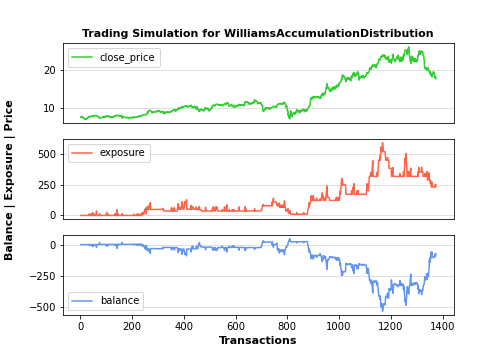
Let’s look at the Williams %R, also known as the Williams Percent Range. It is a type of momentum indicator that moves between 0 and -100 and measures overbought and oversold levels. The Williams %R may be used to find entry and exit points in the market. The indicator is very similar to the Stochastic oscillator and is used in the same way.
from tti.indicators import WilliamsR
wad_indicator = WilliamsR(input_data=df)
Get indicator’s value for a specific date
print(‘\nTechnical Indicator value at 2022-06-15:’, wad_indicator.getTiValue(‘2022-06-15’))
Get the most recent indicator’s value
print(‘\nMost recent Technical Indicator value:’, wad_indicator.getTiValue())
Get signal from indicator
print(‘\nTechnical Indicator signal:’, wad_indicator.getTiSignal())
Show the Graph for the calculated Technical Indicator
wad_indicator.getTiGraph().show()
Save the Graph for the calculated Technical Indicator
wad_indicator.getTiGraph().savefig(‘../TTI/example_wad.png’)
print(‘\nGraph for the calculated fo indicator data, saved.’)
Execute simulation based on trading signals
simulation_data, simulation_statistics, simulation_graph = \
wad_indicator.getTiSimulation(
close_values=df[[‘close’]], max_exposure=None,
short_exposure_factor=1.5)
print(‘\nSimulation Data:\n’, simulation_data)
print(‘\nSimulation Statistics:\n’, simulation_statistics)
Save the Graph for the executed trading signal simulation
simulation_graph.savefig(‘../TTI/simulation_wad.png’)
print(‘\nGraph for the executed trading signal simulation, saved.’)
Technical Indicator value at 2022-06-15: [-65.3594]

Most recent Technical Indicator value: [-93.1373]

Technical Indicator signal: ('hold', 0)

Graph for the calculated fo indicator data, saved.

Simulation Data:
            signal open_trading_action stock_value    exposure portfolio_value  \
Date
2017-01-03   hold                none        7.37         0.0             0.0
2017-01-04   hold                none       7.565         0.0             0.0
2017-01-05   hold                none        7.51         0.0             0.0
2017-01-06   hold                none        7.41         0.0             0.0
2017-01-09   hold                none        7.48         0.0             0.0
...           ...                 ...         ...         ...             ...
2022-06-10   hold                none       18.33  148.005001          -36.66
2022-06-13   hold                none       17.85  148.005001      -35.700001
2022-06-14   hold                none       18.24  148.005001          -36.48
2022-06-15   hold                none   18.290001  148.005001      -36.580002
2022-06-16   hold                none       17.67  148.005001          -35.34

             earnings   balance
Date
2017-01-03        0.0       0.0
2017-01-04        0.0       0.0
2017-01-05        0.0       0.0
2017-01-06        0.0       0.0
2017-01-09        0.0       0.0
...               ...       ...
2022-06-10  40.139992  3.479992
2022-06-13  40.139992  4.439991
2022-06-14  40.139992  3.659993
2022-06-15  40.139992   3.55999
2022-06-16  40.139992  4.799992

[1374 rows x 7 columns]

Simulation Statistics:
 {'number_of_trading_days': 1374, 'number_of_buy_signals': 127, 'number_of_ignored_buy_signals': 0, 'number_of_sell_signals': 130, 'number_of_ignored_sell_signals': 0, 'last_stock_value': 17.67, 'last_exposure': 148.01, 'last_open_long_positions': 3, 'last_open_short_positions': 5, 'last_portfolio_value': -35.34, 'last_earnings': 40.14, 'final_balance': 4.8}

Graph for the executed trading signal simulation, saved.
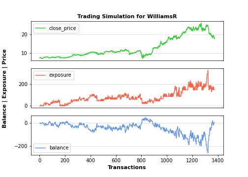
Conclusion
The Trading Technical Indicators (tti) package API
is a python library for calculating more than 60 trading technical indicators from stocks data. The library provides an API for:
- trading technical indicators value calculation
- trading technical indicators graph preparation
- trading signal calculation
- trading simulation based on trading signals
- prices direction prediction based on machine learning algorithms.
The following trading technical indicators are supported by tti:
- Accumulation Distribution Line
- Average True Range
- Bollinger Bands
- Chaikin Money Flow
- Chaikin Oscillator
- Chande Momentum Oscillator
- Commodity Channel Index
- Detrended Price Oscillator
- Directional Movement Index
- Double Exponential Moving Average
- Ease Of Movement
- Envelopes
- Fibonacci Retracement
- Forecast Oscillator
- Ichimoku Cloud
- Intraday Movement Index
- Klinger Oscillator
- Linear Regression Indicator
- Linear Regression Slope
- Market Facilitation Index
- Mass Index
- Median Price
- Momentum
- Exponential Moving Average
- Simple Moving Average
- Time-Series Moving Average
- Triangular Moving Average
- Variable Moving Average
- Moving Average Convergence Divergence
- Negative Volume Index
- On Balance Volume
- Parabolic SAR
- Performance
- Positive Volume Index
- Price And Volume Trend
- Price Channel
- Price Oscillator
- Price Rate Of Change
- Projection Bands
- Projection Oscillator
- Qstick
- Range Indicator
- Relative Momentum Index
- Relative Strength Index
- Relative Volatility Index
- Standard Deviation
- Stochastic Momentum Index
- Fast Stochastic Oscillator
- Slow Stochastic Oscillator
- Swing Index
- Time Series Forecast
- Triple Exponential Moving Average
- Typical Price
- Ultimate Oscillator
- Vertical Horizontal Filter
- Volatility Chaikins
- Volume Oscillator
- Volume Rate Of Change
- Weighted Close
- Wilders Smoothing
- Williams Accumulation Distribution
- Williams %R
Implementation based on the book ‘Technical Analysis from A to Z, Steven B. Achelis’
Validation based on the ‘A to Z Companion Spreadsheet, Steven B. Achelis and Jon C. DeBry’


Leave a comment