In this post, we extend the earlier study by applying FBProphet to Algorithmic Trading using S&P 500 stock for test purposes.
Contents:

The Facebook’s Prophet library is an open-source library designed for automated forecasts for univariate time series datasets such as stock prices. The objective of this test case example is to use Prophet assisted forecasting and algorithmic trading in Python. The data we will be using is the historical daily S&P 500 adjusted close price available in Yahoo Finance.
Importing Libraries
Let’s set the working directory
import os
os.chdir(‘YourPath’) # Set working directory
and import the following libraries
import pandas as pd
import numpy as np
from fbprophet import Prophet
import matplotlib.pyplot as plt
from functools import reduce
%matplotlib inline
import warnings
warnings.filterwarnings(‘ignore’)
plt.style.use(‘seaborn-deep’)
pd.options.display.float_format = “{:,.2f}”.format
Data Preparation
Let’s read the input csv file
stock_price = pd.read_csv(‘^GSPC.csv’,parse_dates=[‘Date’])
stock_price.info()
<class 'pandas.core.frame.DataFrame'>
RangeIndex: 1005 entries, 0 to 1004
Data columns (total 7 columns):
 #   Column     Non-Null Count  Dtype
---  ------     --------------  -----
 0   Date       1005 non-null   datetime64[ns]
 1   Open       1005 non-null   float64
 2   High       1005 non-null   float64
 3   Low        1005 non-null   float64
 4   Close      1005 non-null   float64
 5   Adj Close  1005 non-null   float64
 6   Volume     1005 non-null   int64
dtypes: datetime64[ns](1), float64(5), int64(1)
memory usage: 55.1 KB
Let’s check the statistics
stock_price.describe()

Let’s change the column names
stock_price = stock_price[[‘Date’,’Adj Close’]]
stock_price.columns = [‘ds’, ‘y’]
stock_price.tail(10)

Let’s plot the time-series

Prophet Forecast
Let’s call Prophet() and fit the above stock data by calling the method fit
model = Prophet()
model.fit(stock_price)
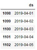
and use make_future_dataframe for forecasting
future = model.make_future_dataframe(100, freq=’d’)
future_boolean = future[‘ds’].map(lambda x : True if x.weekday() in range(0, 5) else False)
future = future[future_boolean]
future.tail()
followed by
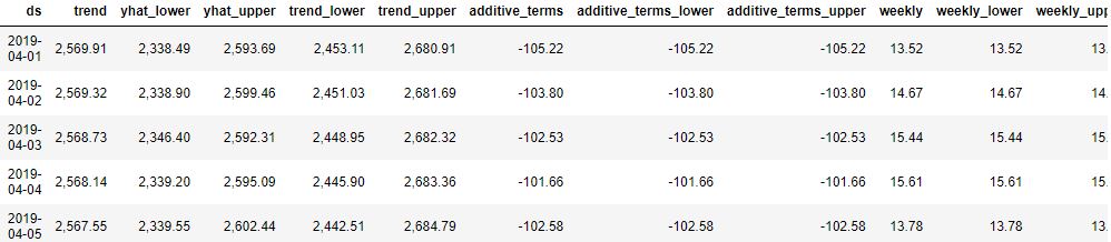
forecast = model.predict(future)
forecast.tail()
Let’s plot the result
model.plot(forecast);

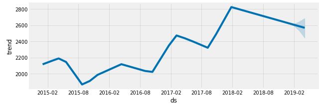
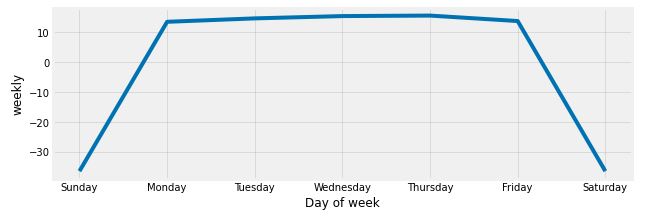
and all components

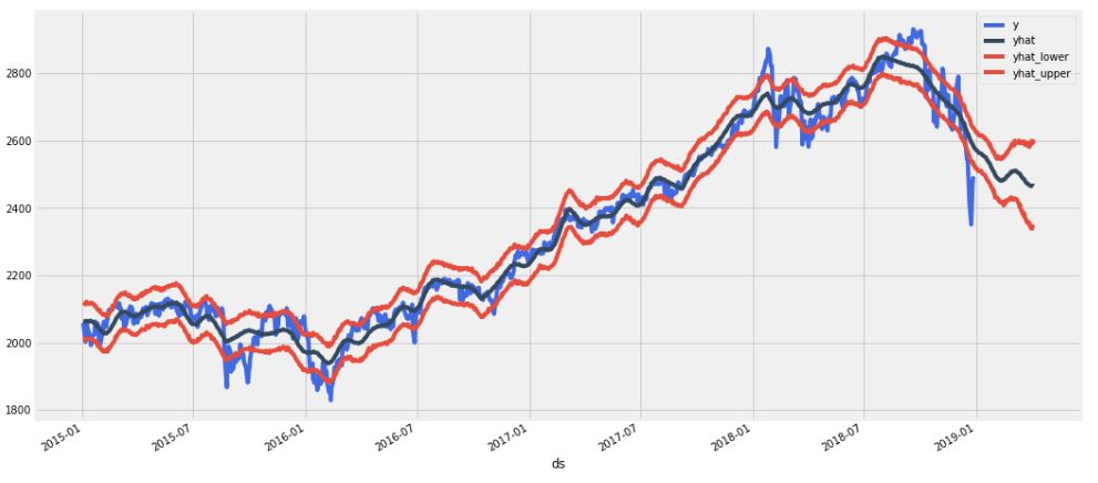
Let’s combine actual data and predictions with lower/upper limits into a single plot
stock_price_forecast = forecast[[‘ds’, ‘yhat’, ‘yhat_lower’, ‘yhat_upper’]]
df = pd.merge(stock_price, stock_price_forecast, on=’ds’, how=’right’)
df.set_index(‘ds’).plot(figsize=(16,8), color=[‘royalblue’, “#34495e”, “#e74c3c”, “#e74c3c”], grid=True);
Forecast Simulations
Let’s see how the above simulations and forecast can be used in trading scenario testing.
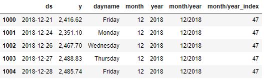
stock_price[‘dayname’] = stock_price[‘ds’].dt.day_name()
stock_price[‘month’] = stock_price[‘ds’].dt.month
stock_price[‘year’] = stock_price[‘ds’].dt.year
stock_price[‘month/year’] = stock_price[‘month’].map(str) + ‘/’ + stock_price[‘year’].map(str)
stock_price = pd.merge(stock_price,
stock_price[‘month/year’].drop_duplicates().reset_index(drop=True).reset_index(),
on=’month/year’,
how=’left’)
stock_price = stock_price.rename(columns={‘index’:’month/year_index’})
stock_price.tail()
Let’s run the loop over each unique month/year in the stock price while fitting the Prophet model and then applying a monthly forecast
loop_list = stock_price[‘month/year’].unique().tolist()
max_num = len(loop_list) – 1
forecast_frames = []
for num, item in enumerate(loop_list):
if  num == max_num:
    pass
else:
    df = stock_price.set_index('ds')[
         stock_price[stock_price['month/year'] == loop_list[0]]['ds'].min():\
         stock_price[stock_price['month/year'] == item]['ds'].max()]

    df = df.reset_index()[['ds', 'y']]

    model = Prophet()
    model.fit(df)

    future = stock_price[stock_price['month/year_index'] == (num + 1)][['ds']]

    forecast = model.predict(future)
    forecast_frames.append(forecast)
INFO:fbprophet:Disabling yearly seasonality. Run prophet with yearly_seasonality=True to override this.
stock_price_forecast = reduce(lambda top, bottom: pd.concat([top, bottom], sort=False), forecast_frames)
stock_price_forecast = stock_price_forecast[[‘ds’, ‘yhat’, ‘yhat_lower’, ‘yhat_upper’]]
stock_price_forecast.to_csv(‘stock_price_forecast.csv’, index=False)
stock_price_forecast = pd.read_csv(‘stock_price_forecast.csv’, parse_dates=[‘ds’])
Let’s merge our data and plot the result
df = pd.merge(stock_price[[‘ds’,’y’, ‘month/year_index’]], stock_price_forecast, on=’ds’)
df[‘Percent Change’] = df[‘y’].pct_change()
df.set_index(‘ds’)[[‘y’, ‘yhat’, ‘yhat_lower’, ‘yhat_upper’]].plot(figsize=(16,8), color=[‘royalblue’, “#34495e”, “#e74c3c”, “#e74c3c”], grid=True)

df.head()

Trading Algorithm
Let’s test the following 4 initial trading algorithms/scenarios:
- Hold: Our bench mark. This is a buy and hold strategy. Meaning we buy the stock and hold it until the end time period.
- Prophet: This strategy is to sell when our forecast indicates a down trend and buy back in when it indicates an upward trend.
- Prophet Thresh: This strategy is to sell only when the stock price fall below our yhat_lower boundary.
- Seasonality: This strategy is to exit the market in August and re-enter in October. This was based on the seasonality chart, as shown above.
These algorithms are as follows
df[‘Hold’] = (df[‘Percent Change’] + 1).cumprod()
df[‘Prophet’] = ((df[‘yhat’].shift(-1) > df[‘yhat’]).shift(1) * (df[‘Percent Change’]) + 1).cumprod()
df[‘Prophet Thresh’] = ((df[‘y’] > df[‘yhat_lower’]).shift(1)* (df[‘Percent Change’]) + 1).cumprod()
df[‘Seasonality’] = ((~df[‘ds’].dt.month.isin([8,9])).shift(1) * (df[‘Percent Change’]) + 1).cumprod()
(df.dropna().set_index(‘ds’)[[‘Hold’, ‘Prophet’, ‘Prophet Thresh’,’Seasonality’]] * 1000).plot(figsize=(16,8), grid=True)
print(f”Hold = {df[‘Hold’].iloc[-1]1000:,.0f}”) print(f”Prophet = {df[‘Prophet’].iloc[-1]1000:,.0f}”)
print(f”Prophet Thresh = {df[‘Prophet Thresh’].iloc[-1]1000:,.0f}”) print(f”Seasonality = {df[‘Seasonality’].iloc[-1]1000:,.0f}”)
Hold = 1,230
Prophet = 1,126
Prophet Thresh = 1,176
Seasonality = 1,269

This is what we get by simulating an initial investment of $1,000. As we can see, the Seasonality and Hold scenarios yield the best outcome.
Summary
- It appears that Prophet works best with time-series data that have strong seasonal effects and several seasons of historical data. It handles outliers well. This observation does support previous studies.
- This project is a real-world realiability test of the serverless investing algorithm based on the AWS Lambda and Facebook Prophet as ML model. The performance efficiency and cost savings are beyond the scope of this study.


Leave a comment