
- The objective of this project is to democratize and advance ML/AI for everyone by building the large open-source showcase of Hugging Face NLP, Streamlit/Dash Jupyter PyGWalker Exploratory Data Analysis (EDA), TensorFlow Keras and Gradio App deployment. There is no better way of showcasing your results than creating an interactive demo to try them out! This allows you to create your ML portfolio, showcase your projects at conferences or to stakeholders, and work collaboratively with other people in the ML ecosystem discussed in the sequel.
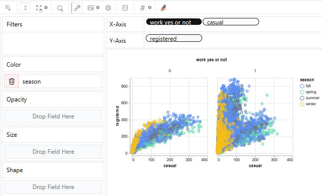
- PyGWalker EDA: NYC bike sharing, Airbnb, USA house prices, and Dutch eHealth.
- Keras Image Classification: CNN CV 5 types of flowers, Iris Flower Predictor and Image Classification with ImageNet algorithms.
- Super Soaker Failures Analysis demonstrated as the Gradio dashboard.
- Supervised ML diabetes prediction and app development using the public-domain dataset.
- We look at the crop recommendation algorithm with Gradio deployment
- Predicting the score of a student based upon the number of study hours.
- Hugging Face NLP/LLM Transformers as pipelines: Image-to-Sketch Conversion, Text Substitution, Story Generation with GPT-2, BigGAN Text-to-Image Demo, French Story Generator using Opus MT and GPT-2, NLP sentence classification, NLP Sentiment Analysis, question answerer, article summarization, text substitution, and EN-to-DE translation.
Table of Contents
- Streamlit/Dash/Jupyter PyGWalker EDA Demo
- Keras Multi-Label Image Classification
- Super Soaker Failures Analysis
- Diabetes Prediction App
- FE+ML SciKit-Learn Diabetes Predictor
- Crop Recommendation
- Student Prediction Score
- Image-to-Sketch Conversion
- Text Substitution
- Story Generation with GPT-2
- BigGAN Text-to-Image Demo
- French Story Generator using Opus MT and GPT-2
- Image Classification with ImageNet
- Iris Flower Predictor
- Hugging Face NLP Sentiment Analysis
- Conclusions
- Explore More
Streamlit/Dash/Jupyter PyGWalker EDA Demo
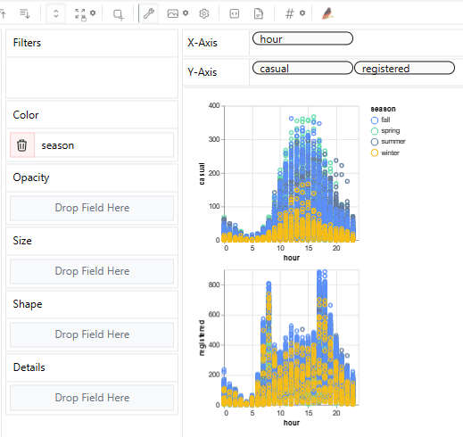
- Let’s look at the Tableau-style PyGWalker app in Streamlit using the dataset bike_sharing_dc.csv
pip install pygwalker
import pygwalker as pyg
import pandas as pd
import streamlit.components.v1 as components
import streamlit as st

# Adjust the width of the Streamlit page
st.set_page_config(
    page_title="Use Pygwalker In Streamlit",
    layout="wide"
)

# Add Title
st.title("Use Pygwalker In Streamlit")

# Import your data
df = pd.read_csv("bike_sharing_dc.csv")

# Generate the HTML using Pygwalker
pyg_html = pyg.to_html(df)

# Embed the HTML into the Streamlit app
components.html(pyg_html, height=1000, scrolling=True)
- streamlit run app_pygwalker.py

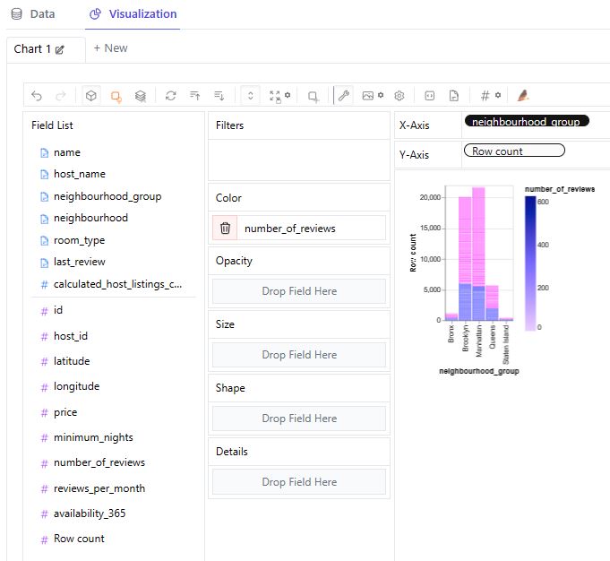
- Airbnb EDA: Implementing PyGWalker Dash UI in Jupyter IDE with gradio/NYC-Airbnb-Open-Data
#https://www.kaggle.com/code/lxy21495892/airbnb-eda-pygwalker-demo

import pygwalker as pyg
import dash
import dash_html_components as html
import dash_dangerously_set_inner_html
import gradio
from datasets import load_dataset
dataset = load_dataset("gradio/NYC-Airbnb-Open-Data", split="train")
df = dataset.to_pandas()
walker = pyg.walk(df, debug=False)
app = dash.Dash(__name__)
html_code = walker.to_html()
app.layout = html.Div([
    dash_dangerously_set_inner_html.DangerouslySetInnerHTML(html_code),
])
if __name__ == '__main__':
    app.run_server(debug=True)


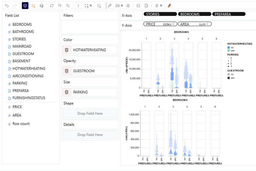
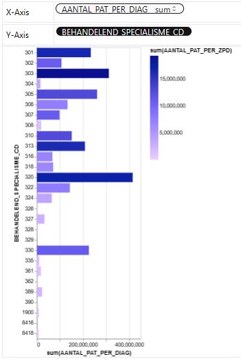
- Let’s look at the House price dataset from Kaggle to showcase the PyGWalker EDA in real estate
import pygwalker as pyg
import pandas as pd
df = pd.read_excel('01_DBC.xlsx')
pyg.walk(df)


- References:
PyGWalker and Dash — Creating a Data Visualization Dashboard In Less Than 20 Lines of Code
PyGWalker Tutorial: A Tableau-Like Python Library for Interactive Data Exploration and Visualization
PyGWalker: A Python Library for Visualizing Pandas Dataframes
You’ll Never Walk Alone: Use Pygwalker to Visualize Data in Jupyter Notebook
PyGWalker 0.1.6. Update: Export Visualizations to Code
A Hands-On Demonstration of the PyGWalker Data Visualization Library – Part 1
Keras Multi-Label Image Classification
- Following the deep learning CNN CV tutorial, we will demonstrate how to easily build an image classification model using Keras and deploy it using Gradio.
- Setting the working directory YOURPATH and importing the key libraries
import os
os.chdir('YOURPATH')    # Set working directory
os. getcwd()
import gradio as gr
import numpy as np
import matplotlib.pyplot as plt
import tensorflow as tf
import PIL
import pathlib
from tensorflow import keras
from tensorflow.keras import layers
- Importing the input images of flowers and setting CNN parameters
import pathlib
dataset_url = "https://storage.googleapis.com/download.tensorflow.org/example_images/flower_photos.tgz"
import tensorflow as tf
data_dir = tf.keras.utils.get_file('flower_photos', origin=dataset_url, untar=True)
data_dir = pathlib.Path(data_dir)
image_count = len(list(data_dir.glob('*/*.jpg')))
print(image_count)
3670
print(os.listdir(data_dir))
['daisy', 'dandelion', 'LICENSE.txt', 'roses', 'sunflowers', 'tulips']
import PIL
roses = list(data_dir.glob('roses/*'))
PIL.Image.open(str(roses[1]))
- Examples of images
import PIL
roses = list(data_dir.glob('roses/*'))
PIL.Image.open(str(roses[1]))

daisy = list(data_dir.glob('daisy/*'))
PIL.Image.open(str(daisy[2]))

- Training images
batch_size = 32
img_height = 180
img_width = 180
train_ds = tf.keras.utils.image_dataset_from_directory(
  data_dir,
  validation_split=0.3,
  subset="training",
  seed=123,
  image_size=(img_height, img_width),
  batch_size=batch_size)
Found 3670 files belonging to 5 classes.
Using 2569 files for training.
- Validation images
val_ds = tf.keras.utils.image_dataset_from_directory(
  data_dir,
  validation_split=0.2,
  subset="validation",
  seed=123,
  image_size=(img_height, img_width),
  batch_size=batch_size)
Found 3670 files belonging to 5 classes.
Using 734 files for validation.
class_names = train_ds.class_names
print(class_names)
['daisy', 'dandelion', 'roses', 'sunflowers', 'tulips']
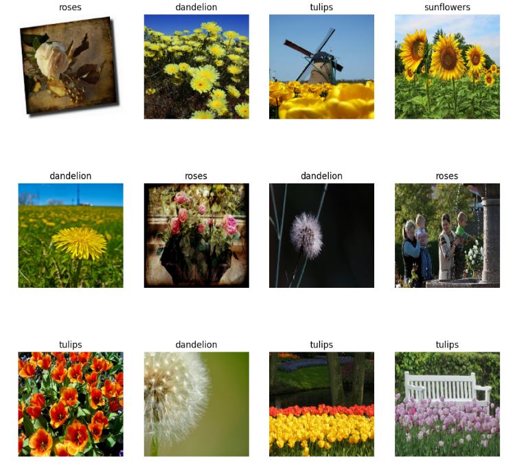
- Plotting training images with 5 labels
import matplotlib.pyplot as plt
plt.figure(figsize=(12, 12))
for images, labels in train_ds.take(1):
  for i in range(12):
    ax = plt.subplot(3, 4, i + 1)
    plt.imshow(images[i].numpy().astype("uint8"))
    plt.title(class_names[labels[i]])
    plt.axis("off")
- Training CNN model
import tensorflow as tf
import keras
from keras import layers

num_classes = len(class_names)
model = keras.Sequential([
  layers.Rescaling(1./255, input_shape=(img_height, img_width, 3)),
  layers.Conv2D(16, 3, padding='same', activation='relu'),
  layers.MaxPooling2D(),
  layers.Conv2D(32, 3, padding='same', activation='relu'),
  layers.MaxPooling2D(),
  layers.Conv2D(64, 3, padding='same', activation='relu'),
  layers.MaxPooling2D(),
  layers.Flatten(),
  layers.Dense(128, activation='relu'),
  layers.Dense(num_classes,activation='softmax')
])
model.compile(optimizer='adam',
              loss=tf.keras.losses.SparseCategoricalCrossentropy(from_logits=True),
              metrics=['accuracy'])
model.summary()
Model: "sequential"
_________________________________________________________________
 Layer (type)                Output Shape              Param #
=================================================================
 rescaling (Rescaling)       (None, 180, 180, 3)       0

 conv2d (Conv2D)             (None, 180, 180, 16)      448

 max_pooling2d (MaxPooling2D  (None, 90, 90, 16)       0
 )

 conv2d_1 (Conv2D)           (None, 90, 90, 32)        4640

 max_pooling2d_1 (MaxPooling  (None, 45, 45, 32)       0
 2D)

 conv2d_2 (Conv2D)           (None, 45, 45, 64)        18496

 max_pooling2d_2 (MaxPooling  (None, 22, 22, 64)       0
 2D)

 flatten (Flatten)           (None, 30976)             0

 dense (Dense)               (None, 128)               3965056

 dense_1 (Dense)             (None, 5)                 645

=================================================================
Total params: 3,989,285
Trainable params: 3,989,285
Non-trainable params: 0
_________________________________________________________________
epochs=20
history = model.fit(
  train_ds,
  validation_data=val_ds,
  epochs=epochs
)
Epoch 1/20
81/81 [==============================] - 22s 272ms/step - loss: 0.8036 - accuracy: 0.6999 - val_loss: 1.0209 - val_accuracy: 0.6063
Epoch 2/20
81/81 [==============================] - 23s 281ms/step - loss: 0.5807 - accuracy: 0.7902 - val_loss: 1.0150 - val_accuracy: 0.6417
Epoch 3/20
81/81 [==============================] - 24s 292ms/step - loss: 0.3573 - accuracy: 0.8758 - val_loss: 1.1478 - val_accuracy: 0.6226
Epoch 4/20
81/81 [==============================] - 24s 293ms/step - loss: 0.2325 - accuracy: 0.9233 - val_loss: 1.5997 - val_accuracy: 0.6104
Epoch 5/20
81/81 [==============================] - 24s 298ms/step - loss: 0.1499 - accuracy: 0.9560 - val_loss: 1.4177 - val_accuracy: 0.6226
Epoch 6/20
81/81 [==============================] - 24s 300ms/step - loss: 0.0902 - accuracy: 0.9755 - val_loss: 1.7358 - val_accuracy: 0.6376
Epoch 7/20
81/81 [==============================] - 24s 295ms/step - loss: 0.0531 - accuracy: 0.9860 - val_loss: 2.0204 - val_accuracy: 0.6226
Epoch 8/20
81/81 [==============================] - 24s 296ms/step - loss: 0.0295 - accuracy: 0.9946 - val_loss: 2.1318 - val_accuracy: 0.6131
Epoch 9/20
81/81 [==============================] - 24s 294ms/step - loss: 0.0135 - accuracy: 0.9981 - val_loss: 2.1777 - val_accuracy: 0.6131
Epoch 10/20
81/81 [==============================] - 25s 302ms/step - loss: 0.0072 - accuracy: 0.9992 - val_loss: 2.2860 - val_accuracy: 0.6090
Epoch 11/20
81/81 [==============================] - 25s 302ms/step - loss: 0.0198 - accuracy: 0.9938 - val_loss: 2.2578 - val_accuracy: 0.6253
Epoch 12/20
81/81 [==============================] - 24s 301ms/step - loss: 0.0224 - accuracy: 0.9942 - val_loss: 2.3855 - val_accuracy: 0.6199
Epoch 13/20
81/81 [==============================] - 25s 306ms/step - loss: 0.0500 - accuracy: 0.9926 - val_loss: 2.0227 - val_accuracy: 0.6144
Epoch 14/20
81/81 [==============================] - 25s 305ms/step - loss: 0.0491 - accuracy: 0.9875 - val_loss: 2.0545 - val_accuracy: 0.6131
Epoch 15/20
81/81 [==============================] - 25s 305ms/step - loss: 0.0667 - accuracy: 0.9805 - val_loss: 2.1308 - val_accuracy: 0.6035
Epoch 16/20
81/81 [==============================] - 25s 307ms/step - loss: 0.0801 - accuracy: 0.9728 - val_loss: 2.1201 - val_accuracy: 0.6090
Epoch 17/20
81/81 [==============================] - 25s 309ms/step - loss: 0.0582 - accuracy: 0.9813 - val_loss: 2.1666 - val_accuracy: 0.5940
Epoch 18/20
81/81 [==============================] - 25s 305ms/step - loss: 0.0146 - accuracy: 0.9965 - val_loss: 2.5094 - val_accuracy: 0.6049
Epoch 19/20
81/81 [==============================] - 25s 307ms/step - loss: 0.0026 - accuracy: 0.9996 - val_loss: 2.5327 - val_accuracy: 0.6035
Epoch 20/20
81/81 [==============================] - 25s 306ms/step - loss: 7.3366e-04 - accuracy: 1.0000 - val_loss: 2.6016 - val_accuracy: 0.6049
- Plotting the key diagnostics
print(history.history.keys())
dict_keys(['loss', 'accuracy', 'val_loss', 'val_accuracy'])

plt.plot(history.history['accuracy'])
plt.plot(history.history['val_accuracy'])
plt.title('model accuracy')
plt.ylabel('accuracy')
plt.xlabel('epoch')
plt.legend(['train', 'test'], loc='upper left')
plt.show()


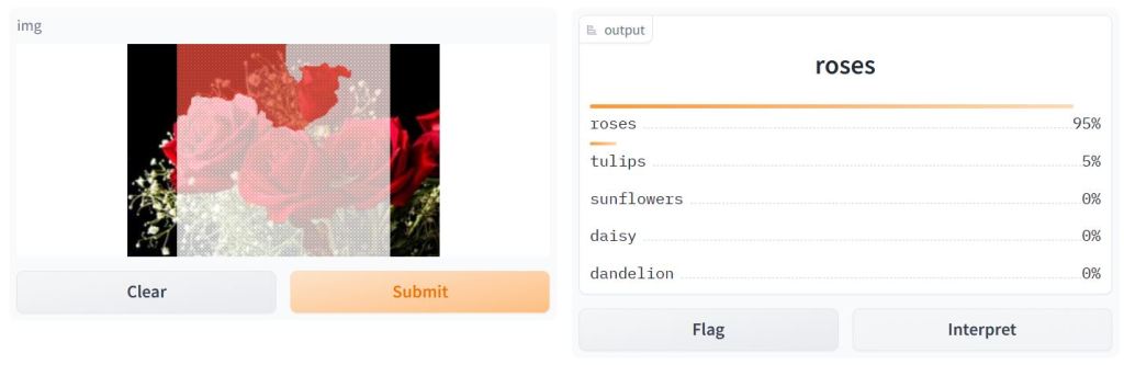
- Deploying the trained CNN model in Gradio
import gradio as gr
image = gr.inputs.Image(shape=(180,180))
label = gr.outputs.Label(num_top_classes=5)

def predict_input_image(img):
  img_4d=img.reshape(-1,180,180,3)
  prediction=model.predict(img_4d)[0]
  return {class_names[i]: float(prediction[i]) for i in range(5)}

import gradio as gr
image = gr.inputs.Image(shape=(180,180))
label = gr.outputs.Label(num_top_classes=5)

gr.Interface(fn=predict_input_image, inputs=image, outputs=label,interpretation='default').launch(debug='True')

Running on local URL
To create a public link, set `share=True` in `launch()`.
Remark: Use via API

Super Soaker Failures Analysis
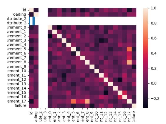
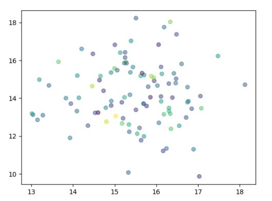
- As an example of UI, let’s consider the super soaker failure analysis dashboard demonstrated as the Gradio workflow
import gradio as gr
import pandas as pd
import datasets
import seaborn as sns
import matplotlib.pyplot as plt

df = datasets.load_dataset("merve/supersoaker-failures")
df = df["train"].to_pandas()
df.dropna(axis=0, inplace=True)

def plot(df):
  plt.scatter(df.measurement_13, df.measurement_15, c = df.loading,alpha=0.5)
  plt.savefig("scatter.png")
  df['failure'].value_counts().plot(kind='bar')
  plt.savefig("bar.png")
  sns.heatmap(df.select_dtypes(include="number").corr())
  plt.savefig("corr.png")
  plots = ["corr.png","scatter.png", "bar.png"]
  return plots

inputs = [gr.Dataframe(label="Supersoaker Production Data")]
outputs = [gr.Gallery(label="Profiling Dashboard", columns=(1,3))]

gr.Interface(plot, inputs=inputs, outputs=outputs, examples=[df.head(100)], title="Supersoaker Failures Analysis Dashboard").launch()


Diabetes Prediction App
- Let’s implement the Diabetes Prediction App using the Gradio tutorial for ML (cf. Gradio documentation) and the SciKit-learn diabetes dataset. Read more here (cf. Colab code and toolkit).
- Importing basic libraries and loading input data
import numpy as np
import pandas as pd
import gradio as gr
import warnings
warnings.filterwarnings('ignore')
from sklearn import datasets
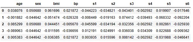
diabetes = datasets.load_diabetes(as_frame=True)
print(type(diabetes['data']))
<class 'pandas.core.frame.DataFrame'>
diabetes['data'].head()
print(diabetes['DESCR'])
.. _diabetes_dataset:

Diabetes dataset
----------------

Ten baseline variables, age, sex, body mass index, average blood
pressure, and six blood serum measurements were obtained for each of n =
442 diabetes patients, as well as the response of interest, a
quantitative measure of disease progression one year after baseline.

**Data Set Characteristics:**

  :Number of Instances: 442

  :Number of Attributes: First 10 columns are numeric predictive values

  :Target: Column 11 is a quantitative measure of disease progression one year after baseline

  :Attribute Information:
      - age     age in years
      - sex
      - bmi     body mass index
      - bp      average blood pressure
      - s1      tc, total serum cholesterol
      - s2      ldl, low-density lipoproteins
      - s3      hdl, high-density lipoproteins
      - s4      tch, total cholesterol / HDL
      - s5      ltg, possibly log of serum triglycerides level
      - s6      glu, blood sugar level

Note: Each of these 10 feature variables have been mean centered and scaled by the standard deviation times the square root of `n_samples` (i.e. the sum of squares of each column totals 1).

Source URL:
https://www4.stat.ncsu.edu/~boos/var.select/diabetes.html

For more information see:
Bradley Efron, Trevor Hastie, Iain Johnstone and Robert Tibshirani (2004) "Least Angle Regression," Annals of Statistics (with discussion), 407-499.
(https://web.stanford.edu/~hastie/Papers/LARS/LeastAngle_2002.pdf)
- Importing additional libraries and trained models
#https://colab.research.google.com/github/bambadij/Cesear-Cypher/blob/main/Diabete_prediction.ipynb#scrollTo=ZT_TFKQMeEjH
#https://github.com/bambadij/gradio_diabete/tree/main/toolkit
#https://github.com/bambadij/gradio_diabete/blob/main/app.py

import gradio as gr
import pandas as pd
import numpy as np
import joblib

#Load scaler ,encoder and model

scaler = joblib.load(r'scaler.joblib')
model = joblib.load(r'model_final.joblib')
encoder = joblib.load(r'encoder.joblib')

# Create a function that applies the ML Pipeline

def predict(Gender,Urea,Cr,HbA1c,Chol,TG,HDL,LDL,VLDL,BMI,age_range):

    # Convertir l'âge en un format numérique
    age_range_mapping = {
        '20-30': 1,
        '30-40': 2,
        '40-50': 3,
        '50-60': 4,
        '60-70': 5,
        '70-80': 6,
        '80-90': 7,
        '90-100': 8,
    }
    age_range_numeric = age_range_mapping.get(age_range, 0)
    #Create a dataframe
    input_df = pd.DataFrame({'Gender':[Gender],
        'Urea':[Urea],
        'Cr':[Cr],
        'HbA1c':[HbA1c],
        'Chol':[Chol],
        'TG':[TG],
        'HDL':[HDL],
        'LDL':[LDL],
        'VLDL':[VLDL],
        'BMI':[BMI],
        'age_range':[age_range_numeric]
        })

    input_df['Urea'] = input_df['Urea'].astype(float)  # Convert  "Urea" in float
    input_df['Gender']=encoder.fit_transform(input_df['Gender'])
    # input_df['CLASS']=encoder.fit_transform(input_df['CLASS'])
    input_df['age_range']=encoder.fit_transform(input_df['age_range'])
    final_df = input_df
    # print("Gender (encoded):", input_df['Gender'])
    # print("Age Range (encoded):", input_df['age_range'])
    #Make prediction using model
    prediction = model.predict(final_df)

    #prediction label
    prediction_label = {
        0: "No Diabetic",
        1: "Predicted Diabetic",
        2: "Diabetic"
    }
    # print(prediction_label)
    print("Prediction (numeric value):", prediction[0])
    print("Prediction (label):", prediction_label[int(prediction[0])])
    return prediction_label[int(prediction[0])]
input_interface=[]

with gr.Blocks() as app:
    Title =gr.Label('Predicting Diabetes App')
    with gr.Row():
        Title

    with gr.Row():
        gr.Markdown("This app predict of Patient to mean Diabete No Diabete or Predicted Diabete")

    with gr.Accordion("Open for information on input"):
        gr.Markdown(""" This app receives the following as inputs and processes them return the prediction on whether a patient given the input will diabeted ,no diabete or predicted.
                        - Gender
                        - Urea: Urea
                        - Cr : Creatinine ratio(Cr)
                        - HbA1c:Sugar Level Blood
                        - Chol : Cholesterol (Chol)
                        - TG :Triglycerides(TG)
                        - HDL :  HDL Cholesterol
                        - LDL:LDL
                        - VLDL:VLDL
                        - BMI :Body Mass Index (BMI)
                        - CLASS : Class (the patient's diabetes disease class may be Diabetic, Non-Diabetic, or Predict-Diabetic)
                        - AGE :Age
                    """)
    with gr.Row():
        with gr.Column():
            input_interface_column_1 = [
                gr.components.Radio(['M','F'],label='Select your gender'),
                gr.components.Dropdown([1 ,2,3,4,5,6,7,8],label='Choose age tranche 1=>(20-30),2=>(30-40),3=>(40-50)...'),
                gr.components.Slider(label='Level urea mg/dl',minimum=0, maximum=100),
                gr.components.Number(label='Level Creatine mg/dl',minimum=0, maximum=100),
                gr.components.Number(label='Sugar Level Blood',minimum=0, maximum=100),
            ]
        with gr.Column():
            input_interface_column_2 = [
                gr.components.Number(label='Level Cholesterol mg/dl',minimum=0, maximum=100),
                gr.components.Number(label='Level Triglycerides mg/dl',minimum=0, maximum=100),
                gr.components.Slider(label='HDL Cholesterol',minimum=0, maximum=100),
                gr.components.Number(label='level LDL',minimum=0, maximum=100),
                gr.components.Number(label='VLDL level',minimum=0, maximum=10),
                gr.components.Slider(label='BMI Body Mass Index',minimum=0, maximum=100),
            ]
    with gr.Row():
        input_interface.extend(input_interface_column_1)
        input_interface.extend(input_interface_column_2)

    with gr.Row():
        predict_btn = gr.Button('Predict',variant="primary")

    #define the output interface
    output_interface = gr.Label(label="Diabetes Status")

    predict_btn.click(fn=predict, inputs=input_interface, outputs=output_interface)

app.launch()


FE+ML SciKit-Learn Diabetes Predictor
- Let’s look at the Random Forest (RF) Feature Engineering (FE) and SciKit-Learn ML diabetes predictions using the public-domain dataset
# Load the data
from sklearn.metrics import accuracy_score
diabetes = pd.read_csv('https://assets.datacamp.com/production/course_1939/datasets/diabetes.csv')
X = diabetes[diabetes.columns[0:-1]]
y = diabetes['diabetes']
# Split into training and test sets
X_train, X_test, y_train, y_test = train_test_split(X, y, random_state=42)
# Import and train a machine learning model
rf = RandomForestClassifier(random_state=42, n_estimators=100)
rf.fit(X_train, y_train)
# Predict on the test data
y_pred = rf.predict(X_test)
# Evaluate the model
accuracy_score(y_test, y_pred)
0.734375
importances = rf.feature_importances_
importances
array([0.07449143, 0.27876091, 0.08888318, 0.07157507, 0.07091345,
0.15805822, 0.11822478, 0.13909297])
# Find index of those with highest importance, sorted from largest to smallest:
indices = np.argsort(importances)[::-1]
for f in range(X.shape[1]):
print(f'{X.columns[indices[f]]}: {np.round(importances[indices[f]],2)}')
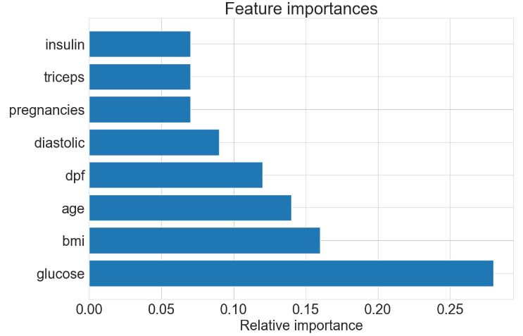
glucose: 0.28
bmi: 0.16
age: 0.14
dpf: 0.12
diastolic: 0.09
pregnancies: 0.07
triceps: 0.07
insulin: 0.07
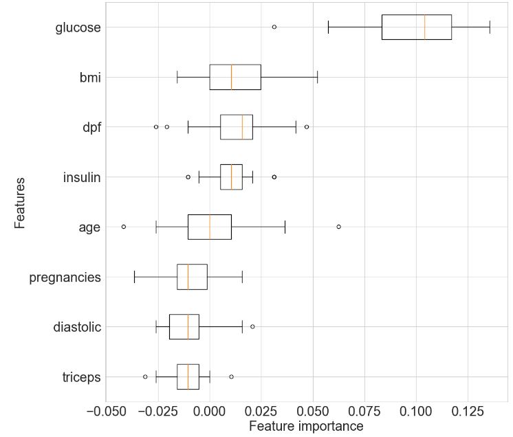
- Plotting RF FE
# Set the figure size and the number of decimal places to round the importances to
fig_size = (12, 8)
decimals = 2
plt.rcParams.update({'font.size': 22})
# Create the horizontal bar plot of feature importances
f, ax = plt.subplots(figsize=fig_size)
plt.barh(X.columns[indices], np.round(importances[indices], decimals))
ax.set_xlabel("Relative importance")
ax.set_title("Feature importances")
plt.show()
# Import the permutation_importance function
from sklearn.inspection import permutation_importance

# Calculate feature importances using permutation importance
n_repeats = 30
random_state = 0
r = permutation_importance(rf, X_test, y_test,
                            n_repeats=n_repeats,
                            random_state=random_state)
for i in r.importances_mean.argsort()[::-1]:
    print(f"{X_test.columns[i]:<8}"
    f"{r.importances_mean[i]:.3f}"
    f" +/- {r.importances_std[i]:.3f}")

glucose 0.098 +/- 0.026
bmi     0.013 +/- 0.020
dpf     0.013 +/- 0.016
insulin 0.010 +/- 0.011
age     0.000 +/- 0.020
pregnancies-0.009 +/- 0.014
diastolic-0.010 +/- 0.011
triceps -0.012 +/- 0.009
# Get the sorted indices of the features according to mean importance
r_sorted_idx = r.importances_mean.argsort()

# Set the figure size
fig_size = (12, 12)
plt.rcParams.update({'font.size': 22})
# Create a boxplot
fig, ax = plt.subplots(figsize=fig_size)
ax.boxplot(
    r.importances[r_sorted_idx].T,
    vert=False,
    labels=X_test.columns[r_sorted_idx],
)

# Add axis labels
plt.xlabel('Feature importance')
plt.ylabel('Features')

plt.show()
- Partial dependence plot for the “glucose” feature
# Import the PartialDependenceDisplay function
from sklearn.inspection import PartialDependenceDisplay

# Set the figure size
fig_size = (10, 6)
plt.rcParams.update({'font.size': 22})
# Create a plot of partial dependence for the 'glucose' feature
f, ax = plt.subplots(figsize=fig_size)
PartialDependenceDisplay.from_estimator(rf, X_train, ['glucose'], kind='both', subsample=50,
                                       ax=ax)

# Add a title to the plot
plt.title('Partial dependence plot for the "glucose" feature')

plt.show()

- Partial dependence plot for the “bmi” feature
f, ax = plt.subplots(figsize=(10,6))
plt.rcParams.update({'font.size': 22})
PartialDependenceDisplay.from_estimator(rf, X_train, ['bmi'], kind='both', subsample=50,
                                       ax=ax)
plt.show()

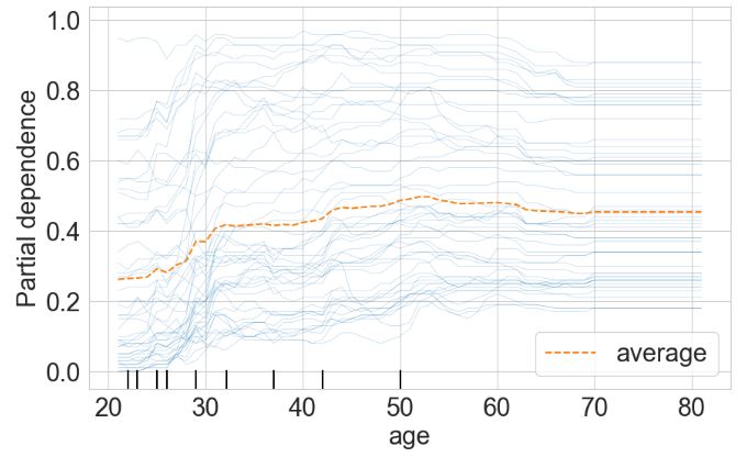
- Partial dependence plot for the “age” feature
f, ax = plt.subplots(figsize=(10,6))
plt.rcParams.update({'font.size': 22})
PartialDependenceDisplay.from_estimator(rf, X_train, ['age'], kind='both',  subsample=50,
                                       ax=ax)
plt.show()
- Partial dependence plot for the “bmi-glucose” features
f, ax = plt.subplots(figsize=(12,8))
plt.rcParams.update({'font.size': 22})
PartialDependenceDisplay.from_estimator(rf, X_train, [('glucose', 'bmi')], kind='average',  subsample=50,
                                        ax=ax)
plt.show()

- Implementing the ML diabetes predictor App in Gradio
#https://www.kaggle.com/code/alexanderlundervold/2023-dat158-1-1-simple-examples-ipynb
import gradio as gr
def predict_diabetes(age, bmi, glucose):
    """
    Predicts whether a person is diabetic or non-diabetic based on their age, BMI, and glucose level.

    Args:
        age (float): The person's age in years.
        bmi (float): The person's body mass index (BMI).
        glucose (float): The person's glucose level in mg/dL.

    Returns:
        str: "Diabetic" if the person is predicted to be diabetic, "Non-diabetic" otherwise.
    """

    # Use the mean values for the unused features
    mean_insulin = diabetes.insulin.mean()
    mean_dpf = diabetes.dpf.mean()
    mean_pregnancies = diabetes.pregnancies.mean()
    mean_triceps = diabetes.triceps.mean()
    mean_diastolic = diabetes.diastolic.mean()

    # Reshape the input data for prediction
    input_data = np.array([mean_pregnancies, glucose, mean_diastolic, mean_triceps,
                           mean_insulin, bmi, mean_dpf, age]).reshape(1, -1)

    # Get the prediction
    prediction = rf.predict(input_data)

    # Return the result
    return "Diabetic" if prediction[0] == 1 else "Non-diabetic"
# Set the minimum, maximum, and default values for the sliders
age_min, age_max, age_default = 0, 100, 30
bmi_min, bmi_max, bmi_default = 15, 50, 25
glucose_min, glucose_max, glucose_default = 0, 200, 100

# Create the interface
iface = gr.Interface(
    fn=predict_diabetes,
    inputs=[
        gr.components.Slider(minimum=age_min, maximum=age_max, value=age_default, label="Age"),
        gr.components.Slider(minimum=bmi_min, maximum=bmi_max, value=bmi_default, label="BMI"),
        gr.components.Slider(minimum=glucose_min, maximum=glucose_max, value=glucose_default, label="Glucose Level")
    ],
    outputs=gr.components.Textbox(label="Prediction"),
    title="Diabetes Predictor",
    description="""Enter your age, BMI, and glucose level to predict whether you are diabetic or non-diabetic.
    Data source: Pima Indians Diabetes Database; Model: Random Forest Classifier""",
)

# Launch the interface
iface.launch(share=True)

Crop Recommendation
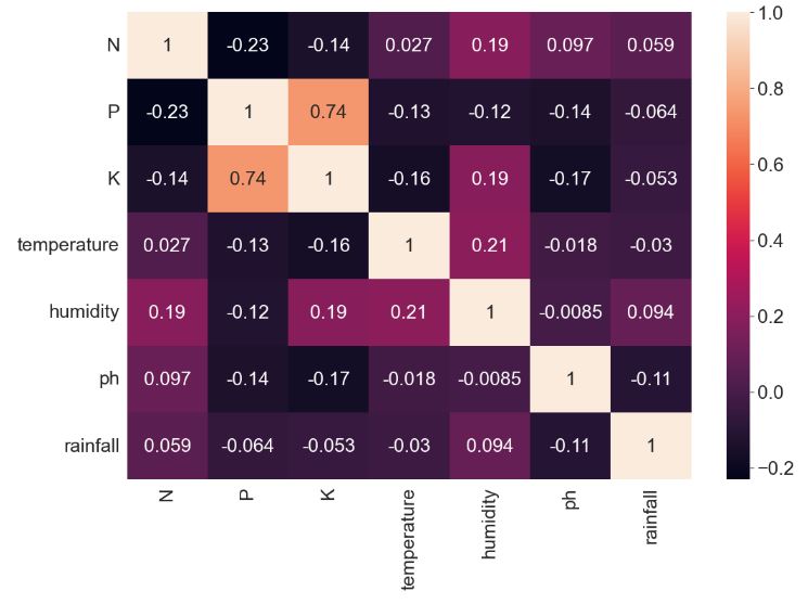
- Let’s look at the crop recommendation algorithm with Gradio deployment
import pandas as pd
import numpy as np
import seaborn as sns
from matplotlib import pyplot as plt
df = pd.read_csv("Crop_recommendation.csv")
plt.figure(figsize=(12,8))
plt.rcParams.update({'font.size': 18})
sns.heatmap(df.corr(),annot=True)
- Training, testing and validating several ML models
features = df[['N','P','K','temperature','humidity','ph','rainfall']]
target = df['label']
labels = df['label']
acc=[]
model = []
from sklearn.model_selection import train_test_split
xtrain,xtest,ytrain,ytest = train_test_split(features,target,random_state=42,test_size=0.2)
- Decision Tree Classifier
from sklearn.tree import DecisionTreeClassifier
from sklearn import metrics
from sklearn.metrics import classification_report
dt = DecisionTreeClassifier(criterion="entropy",random_state=42,max_depth=5)
dt.fit(xtrain,ytrain)
predicted_values = dt.predict(xtest)
x = metrics.accuracy_score(ytest, predicted_values)
acc.append(x)
model.append('Decision Tree')
print("DecisionTrees's Accuracy is: ", x*100)

print(classification_report(ytest,predicted_values))

DecisionTrees's Accuracy is:  86.5909090909091
              precision    recall  f1-score   support

       apple       1.00      1.00      1.00        23
      banana       1.00      1.00      1.00        21
   blackgram       0.61      1.00      0.75        20
    chickpea       1.00      0.96      0.98        26
     coconut       0.96      0.96      0.96        27
      coffee       1.00      1.00      1.00        17
      cotton       1.00      1.00      1.00        17
      grapes       1.00      1.00      1.00        14
        jute       0.63      0.96      0.76        23
 kidneybeans       0.00      0.00      0.00        20
      lentil       0.42      1.00      0.59        11
       maize       1.00      1.00      1.00        21
       mango       1.00      1.00      1.00        19
   mothbeans       0.00      0.00      0.00        24
    mungbean       1.00      1.00      1.00        19
   muskmelon       1.00      1.00      1.00        17
      orange       1.00      1.00      1.00        14
      papaya       1.00      0.87      0.93        23
  pigeonpeas       0.59      1.00      0.74        23
 pomegranate       1.00      0.91      0.95        23
        rice       0.92      0.63      0.75        19
  watermelon       1.00      1.00      1.00        19

    accuracy                           0.87       440
   macro avg       0.82      0.88      0.84       440
weighted avg       0.82      0.87      0.83       440
from sklearn.model_selection import cross_val_score
score = cross_val_score(dt, features, target,cv=5)
score
array([0.93636364, 0.91136364, 0.92045455, 0.87272727, 0.93636364])
import pickle as pk
pk.dump(dt,open('Decision Tree','wb'))
- Gaussian NB
from sklearn.naive_bayes import GaussianNB
gnb = GaussianNB()

gnb.fit(xtrain,ytrain)

predicted_values = gnb.predict(xtest)
x = metrics.accuracy_score(ytest, predicted_values)
acc.append(x)
model.append('Naive Bayes')
print("Naive Bayes's Accuracy is: ", x)

print(classification_report(ytest,predicted_values))

Naive Bayes's Accuracy is:  0.9954545454545455
              precision    recall  f1-score   support

       apple       1.00      1.00      1.00        23
      banana       1.00      1.00      1.00        21
   blackgram       1.00      1.00      1.00        20
    chickpea       1.00      1.00      1.00        26
     coconut       1.00      1.00      1.00        27
      coffee       1.00      1.00      1.00        17
      cotton       1.00      1.00      1.00        17
      grapes       1.00      1.00      1.00        14
        jute       0.92      1.00      0.96        23
 kidneybeans       1.00      1.00      1.00        20
      lentil       1.00      1.00      1.00        11
       maize       1.00      1.00      1.00        21
       mango       1.00      1.00      1.00        19
   mothbeans       1.00      1.00      1.00        24
    mungbean       1.00      1.00      1.00        19
   muskmelon       1.00      1.00      1.00        17
      orange       1.00      1.00      1.00        14
      papaya       1.00      1.00      1.00        23
  pigeonpeas       1.00      1.00      1.00        23
 pomegranate       1.00      1.00      1.00        23
        rice       1.00      0.89      0.94        19
  watermelon       1.00      1.00      1.00        19

    accuracy                           1.00       440
   macro avg       1.00      1.00      1.00       440
weighted avg       1.00      1.00      1.00       440
score = cross_val_score(gnb,features,target,cv=5)
score
array([0.99772727, 0.99545455, 0.99545455, 0.99545455, 0.99090909])
pk.dump(gnb,open('Guassian Naive Bayes','wb'))
- SVM/SVC
from sklearn.svm import SVC
# data normalization with sklearn
from sklearn.preprocessing import MinMaxScaler
# fit scaler on training data
norm = MinMaxScaler().fit(xtrain)
x_train_norm = norm.transform(xtrain)
# transform testing dataabs
x_test_norm = norm.transform(xtest)
SVM = SVC(kernel='poly', degree=3, C=1)
SVM.fit(x_train_norm,ytrain)
predicted_values = SVM.predict(x_test_norm)
x = metrics.accuracy_score(ytest, predicted_values)
acc.append(x)
model.append('SVM')
print("SVM's Accuracy is: ", x)

print(classification_report(ytest,predicted_values))

SVM's Accuracy is:  0.9636363636363636
              precision    recall  f1-score   support

       apple       1.00      1.00      1.00        23
      banana       1.00      1.00      1.00        21
   blackgram       0.90      0.95      0.93        20
    chickpea       1.00      1.00      1.00        26
     coconut       1.00      1.00      1.00        27
      coffee       1.00      0.94      0.97        17
      cotton       0.94      1.00      0.97        17
      grapes       1.00      1.00      1.00        14
        jute       0.80      0.87      0.83        23
 kidneybeans       0.91      1.00      0.95        20
      lentil       0.79      1.00      0.88        11
       maize       1.00      0.95      0.98        21
       mango       1.00      1.00      1.00        19
   mothbeans       1.00      0.92      0.96        24
    mungbean       1.00      1.00      1.00        19
   muskmelon       1.00      1.00      1.00        17
      orange       1.00      1.00      1.00        14
      papaya       0.96      1.00      0.98        23
  pigeonpeas       1.00      0.83      0.90        23
 pomegranate       1.00      1.00      1.00        23
        rice       0.88      0.79      0.83        19
  watermelon       1.00      1.00      1.00        19

    accuracy                           0.96       440
   macro avg       0.96      0.97      0.96       440
weighted avg       0.97      0.96      0.96       440
score = cross_val_score(SVM,features,target,cv=5)
score

array([0.97954545, 0.975     , 0.98863636, 0.98863636, 0.98181818])

pk.dump(SVM,open('SVM','wb'))
- Logistic Regression
from sklearn.linear_model import LogisticRegression

LogReg = LogisticRegression(random_state=2)

LogReg.fit(xtrain,ytrain)

predicted_values = LogReg.predict(xtest)

x = metrics.accuracy_score(ytest, predicted_values)
acc.append(x)
model.append('Logistic Regression')
print("Logistic Regression's Accuracy is: ", x)

print(classification_report(ytest,predicted_values))

Logistic Regression's Accuracy is:  0.9454545454545454
              precision    recall  f1-score   support

       apple       1.00      1.00      1.00        23
      banana       0.95      1.00      0.98        21
   blackgram       0.83      0.75      0.79        20
    chickpea       1.00      1.00      1.00        26
     coconut       1.00      1.00      1.00        27
      coffee       0.94      1.00      0.97        17
      cotton       0.80      0.94      0.86        17
      grapes       1.00      1.00      1.00        14
        jute       0.91      0.87      0.89        23
 kidneybeans       1.00      0.95      0.97        20
      lentil       0.83      0.91      0.87        11
       maize       0.94      0.76      0.84        21
       mango       0.95      1.00      0.97        19
   mothbeans       0.85      0.92      0.88        24
    mungbean       0.95      1.00      0.97        19
   muskmelon       1.00      1.00      1.00        17
      orange       1.00      1.00      1.00        14
      papaya       0.95      0.91      0.93        23
  pigeonpeas       0.95      0.91      0.93        23
 pomegranate       1.00      1.00      1.00        23
        rice       0.89      0.89      0.89        19
  watermelon       1.00      1.00      1.00        19

    accuracy                           0.95       440
   macro avg       0.94      0.95      0.94       440
weighted avg       0.95      0.95      0.94       440

pk.dump(LogReg,open('LogisticRegression','wb'))
- Random Forest Classifier
from sklearn.ensemble import RandomForestClassifier

RF = RandomForestClassifier(n_estimators=20, random_state=0)
RF.fit(xtrain,ytrain)

predicted_values = RF.predict(xtest)

x = metrics.accuracy_score(ytest, predicted_values)
acc.append(x)
model.append('RF')
print("RF's Accuracy is: ", x)

RF's Accuracy is:  0.9931818181818182
- ML accuracy comparison bar plot
plt.figure(figsize=[10,5])
plt.rcParams.update({'font.size': 22})
plt.title('Accuracy Comparison')
plt.xlabel('Accuracy')
plt.ylabel('Algorithm')
sns.barplot(x = acc,y = model,palette='dark')

accuracy_models = dict(zip(model, acc))
for k, v in accuracy_models.items():
    print (k, '-->', v)
Decision Tree --> 0.865909090909091
Naive Bayes --> 0.9954545454545455
SVM --> 0.9636363636363636
Logistic Regression --> 0.9454545454545454
RF --> 0.9931818181818182

data = np.array([[104,18, 30, 23.603016, 60.3, 6.7, 140.91]])
prediction = RF.predict(data)
print(prediction)
['coffee']

import gradio as gr
def crop_recom(N,P,K,tem,hum,ph,rain):
    crop = RF.predict([[N,P,K,tem,hum,ph,rain]])
    return crop
- Run Gradio app
interface = gr.Interface(
  fn =crop_recom, #function
  inputs = ['number','number','number','number','number','number','number'],
  outputs = ['text']


).launch(share=False)

Student Prediction Score
- Predicting the Score of a student based upon the number of study hours.
#https://medium.com/@kalyaniavhale7/tutorial-on-gradio-library-ecb8055923a1
import gradio as gr
import pandas as pd
import numpy as np
from sklearn.linear_model import LinearRegression
#load the dataset to pandas dataframe
URL = "http://bit.ly/w-data"
student_data = pd.read_csv(URL)
#Prepare data
X = student_data.copy()
y = student_data['Scores']
del X['Scores']
#create a machine learning model and train it
lineareg = LinearRegression()
lineareg.fit(X,y)
print('Accuracy score : ',lineareg.score(X,y),'\n')
#now the model has been trained well let test it
#function to predict the input hours
def predict_score(hours):
    hours = np.array(hours)
    pred_score = lineareg.predict(hours.reshape(-1,1))
    return np.round(pred_score[0], 2)
input = gr.inputs.Number(label='Number of Hours studied')
output = gr.outputs.Textbox(label='Predicted Score')
gr.Interface( fn=predict_score,
              inputs=input,
              outputs=output).launch();

Accuracy score :  0.9529481969048356

Running on local URL:

To create a public link, set `share=True` in `launch()`.

Image-to-Sketch Conversion
- Converting RGB image to sketch using opencv library
#https://medium.com/@kalyaniavhale7/tutorial-on-gradio-library-ecb8055923a1
import cv2
import gradio as gr
def convert_photo_to_Sketch(image):
  img = cv2.resize(image, (256, 256))
  #convert image to RGB from BGR
  RGB_img = cv2.cvtColor(img,cv2.COLOR_BGR2RGB)
  #convert imge to grey
  grey_img=cv2.cvtColor(RGB_img, cv2.COLOR_BGR2GRAY)
  #invert grey scale image
  invert_img=255-grey_img
  #Gaussian fun to blur the image
  blur_img=cv2.GaussianBlur(invert_img, (21,21),0)
  #invert the blur image
  inverted_blurred_img = 255 - blur_img
  #skecth the image
  sketch_img=cv2.divide(grey_img,inverted_blurred_img, scale=256.0)
  rgb_sketch=cv2.cvtColor(sketch_img, cv2.COLOR_BGR2RGB)
  #return the final sketched image
  return rgb_sketch

#built interface with gradio to test the function
imagein = gr.inputs.Image(label='Original Image')
imageout =  gr.outputs.Image(label='Sketched Image',type='pil')
gr.Interface(fn=convert_photo_to_Sketch, inputs=imagein, outputs=imageout,title='Convert RGB Image to Sketch').launch();

Text Substitution
- Let’s perform text substitution in Gradio, e.g. text.replace(‘World’, ‘Databricks’)
import gradio as gr
import time

def replace(text):
    return text.replace('World', 'Databricks')

gr.Interface(fn=replace,
             inputs='textbox',
             outputs='textbox').launch(share=True);

Story Generation with GPT-2
- Let’s examine story generation with GPT-2
import gradio as gr

description = "Story generation with GPT-2"

title = "Generate your own story"

examples = [["It was the best of time it was the worst of times. It was difficult for me to love someone. Until I met her. It happened on a rainy evening."]]


interface = gr.Interface.load("huggingface/pranavpsv/gpt2-genre-story-generator",
                              description=description,
                              examples=examples)

interface.launch(share=True);

Fetching model from: https://huggingface.co/pranavpsv/gpt2-genre-story-generator
Running on local URL:

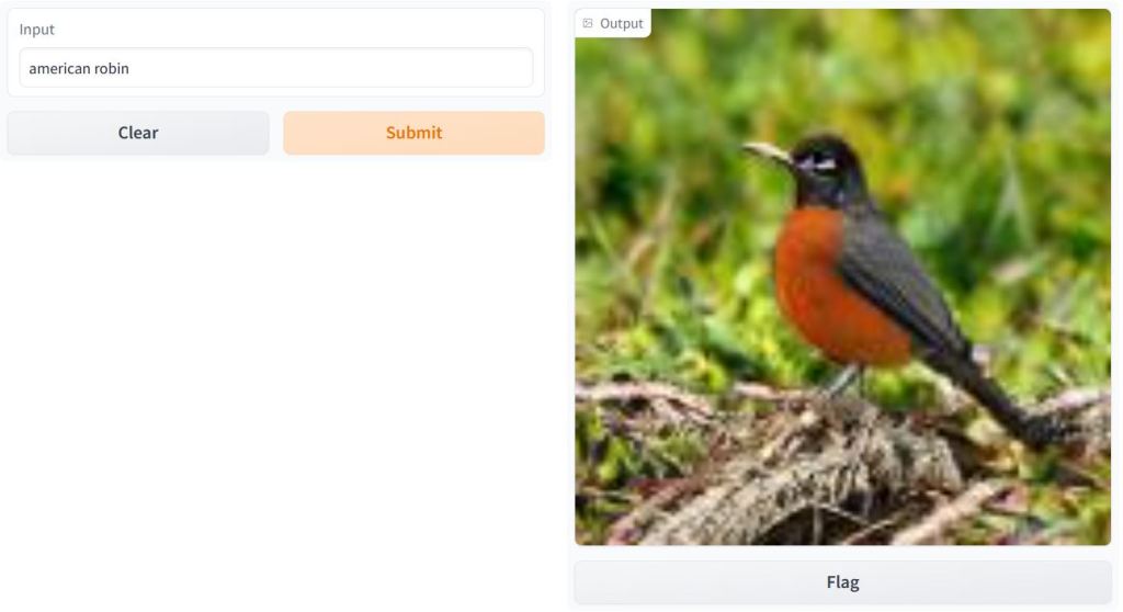
BigGAN Text-to-Image Demo
- Let’s discuss the Sarus tech portfolio – a TensorFlow 2 implementation of BigGAN deep neural network, viz. the BigGAN ImageNet text-to-image transformation.
import gradio as gr
description = "BigGAN text-to-image demo."
title = "BigGAN ImageNet"
interface = gr.Interface.load("huggingface/osanseviero/BigGAN-deep-128",
            description=description,
            title = title,
            examples=[["american robin"]]
)
interface.launch(share=True)

Fetching model from: https://huggingface.co/osanseviero/BigGAN-deep-128
Running on local URL:
BigGAN text-to-image demo: American robin and tiger.
French Story Generator using Opus MT and GPT-2
- LLM integration test: let’s try to generate our own D&D story using Opus MT and GPT-2
import gradio as gr
from gradio.mix import Series

description = "Generate your own D&D story!"
title = "French Story Generator using Opus MT and GPT-2"
translator_fr = gr.Interface.load("huggingface/Helsinki-NLP/opus-mt-fr-en")
story_gen = gr.Interface.load("huggingface/pranavpsv/gpt2-genre-story-generator")
translator_en = gr.Interface.load("huggingface/Helsinki-NLP/opus-mt-en-fr")
examples = [["L'aventurier est approché par un mystérieux étranger, pour une nouvelle quête."]]

Series(translator_fr, story_gen, translator_en, description = description,
        title = title,
        examples=examples, inputs = gr.inputs.Textbox(lines = 10)).launch(share=True)

Fetching model from: https://huggingface.co/Helsinki-NLP/opus-mt-fr-en
Fetching model from: https://huggingface.co/pranavpsv/gpt2-genre-story-generator
Fetching model from: https://huggingface.co/Helsinki-NLP/opus-mt-en-fr
Running on local URL:

Input: The adventurer is approached by a mysterious stranger for a new quest.
Output: L’aventurier est approché par un mystérieux étranger pour une nouvelle quête. De son chemin, l’aventurier rencontre la mystérieuse baronne, Tzachi, mais la rencontre dans le processus.
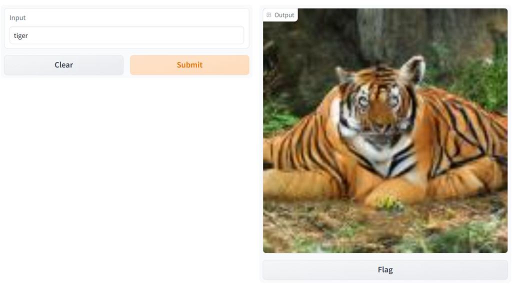
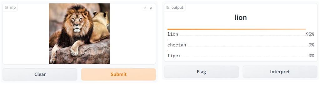
Image Classification with ImageNet
- Let’s download the human-readable labels for ImageNet to perform image classification
#https://www.kaggle.com/code/abidlabs/gradio-inceptionnet-demo
import gradio as gr
import tensorflow as tf
import requests
import urllib

inception_net = tf.keras.applications.InceptionV3() # load the model

# Download human-readable labels for ImageNet.
response = requests.get("https://git.io/JJkYN")
labels = response.text.split("\n")
# Download example image
urllib.request.urlretrieve("https://git.io/JtScc", "lion.jpg")

def classify_image(inp):
    inp = inp[None, ...]  # Add batch dimension
    inp = tf.keras.applications.inception_v3.preprocess_input(inp)
    prediction = inception_net.predict(inp).flatten()
    return {labels[i]: float(prediction[i]) for i in range(1000)}

# Create the Gradio Interface
image = gr.inputs.Image(shape=(299, 299))
label = gr.outputs.Label(num_top_classes=3)

gr.Interface(fn=classify_image, inputs=image, outputs=label, examples=[["lion.jpg"]], interpretation="default").launch(share=True);

Running on local URL:
Image classification examples: lion, dog, and cat.


Iris Flower Predictor
- Let’s use the Iris dataset to predict whether an Iris flower is a Versicolor, Virginica, or Setosa
#https://www.kaggle.com/code/alexanderlundervold/simple-gradio-kaggle-example
import numpy as np
import pandas as pd
import matplotlib.pyplot as plt

import gradio as gr
# Load the data and split into data and labels
from sklearn.datasets import load_iris
iris_dataset = load_iris()
# We use only The 0'th and 1'st columns.
# These correspond to sepal length and width.
X = iris_dataset['data'][:, [0, 1]]
y = iris_dataset['target']

# Split into training and test sets
from sklearn.model_selection import train_test_split
X_train, X_test, y_train, y_test = train_test_split(X, y, random_state=42)

# Import and train a machine learning model
from sklearn.ensemble import RandomForestClassifier
rf = RandomForestClassifier(random_state=42, n_estimators=100)
rf.fit(X_train, y_train)

# Predict on the test data
y_pred = rf.predict(X_test)

# Evaluate the model
from sklearn.metrics import accuracy_score
print(accuracy_score(y_test, y_pred))
0.7894736842105263
def predict_flower(sepal_length, sepal_width):
    """
    Predicts whether an Iris flower is a Versicolor, Virginica, or Setosa.

    Args:
        sepal_length (float): The flower's average sepal length in cm.
        sepal_width (float): The flower's average sepal width in cm.

    Returns:
        str: "Virginica", "Setosa", or "Versicolor".
    """

    # Reshape the input data for prediction
    input_data = np.array([sepal_length, sepal_width]).reshape(1, -1)

    # Get the prediction
    prediction = rf.predict(input_data)

    # Return the result
    if prediction[0] == 0:
        return "Setosa"
    elif prediction[0] == 1:
        return "Versicolor"
    elif prediction[0] == 2:
        return "Virginica"
    else:
        raise Exception
# Set the minimum, maximum, and default values for the sliders
# This is optional
sl_min = X_train[:,0].min().round(2)
sl_max = X_train[:,0].max().round(2)
sl_default = X_train[:,0].mean().round(2)

sw_min = X_train[:,1].min().round(2)
sw_max = X_train[:,1].max().round(2)
sw_default = X_train[:,1].mean().round(2)

# Create the interface
iface = gr.Interface(
    fn=predict_flower,
    inputs=[
        gr.components.Slider(minimum=sl_min, maximum=sl_max,
                             value=sl_default, label="Sepal length"),
        gr.components.Slider(minimum=sw_min, maximum=sw_max,
                             value=sw_default, label="Sepal width"),
    ],
    outputs=gr.components.Textbox(label="Prediction"),
    title="Flower Predictor",
    description="""Enter your measurement of Sepal Length and Sepal Width to
    predict the class of flower.
    Data source: Iris Flower Dataset; Model: Random Forest Classifier""",
)

# Launch the interface
iface.launch(share=True,debug=True)
Running on local URL:

Hugging Face NLP Sentiment Analysis
- Let’s invoke the Hugging Face Transformers to perform NLP Sentiment Analysis as a pipeline
from transformers import pipeline
classifier = pipeline('sentiment-analysis')
- QC test examples of the classifier
classifier("I hate that movie and the cast was bad ")
[{'label': 'NEGATIVE', 'score': 0.9996799230575562}]

classifier("The meal was delicious ")
[{'label': 'POSITIVE', 'score': 0.9998772144317627}]

classifier("That is an ordinary burger ")
[{'label': 'NEGATIVE', 'score': 0.9684451818466187}]
- Initializing BertForSequenceClassification
classifier2 = pipeline('sentiment-analysis', model='bert-base-uncased')
- QC test examples of the classifier2
classifier2("I loved that movie and the cast was good ")
[{'label': 'LABEL_1', 'score': 0.5746493935585022}]

results = classifier(["We are very happy to show you the 🤗 Transformers library.",
           "We hope you don't hate it."])
for i in results:
    print(f"{i['label']}, {round(i['score'],2)}")
POSITIVE, 1.0
NEGATIVE, 0.53
- Initializing and QC testing the text generator
generator = pipeline('text-generation')

print(generator("As far as I am concerned, I will",))
[{'generated_text': 'As far as I am concerned, I will not become a member: if you want, I will show you more images of my real life.\n\nI will not use your personal pictures. When I use your picture on something (for example a'}]
- Fill-mask: initializing distilroberta-base and revision ec58a5b (https://huggingface.co/distilroberta-base) with the QC test
unmasker = pipeline("fill-mask")
from pprint import pprint
pprint(unmasker(f"HuggingFace is creating a {unmasker.tokenizer.mask_token} that the community uses to solve NLP tasks."))
[{'score': 0.1792752891778946,
  'sequence': 'HuggingFace is creating a tool that the community uses to solve '
              'NLP tasks.',
  'token': 3944,
  'token_str': ' tool'},
 {'score': 0.113493911921978,
  'sequence': 'HuggingFace is creating a framework that the community uses to '
              'solve NLP tasks.',
  'token': 7208,
  'token_str': ' framework'},
 {'score': 0.05243545398116112,
  'sequence': 'HuggingFace is creating a library that the community uses to '
              'solve NLP tasks.',
  'token': 5560,
  'token_str': ' library'},
 {'score': 0.034935273230075836,
  'sequence': 'HuggingFace is creating a database that the community uses to '
              'solve NLP tasks.',
  'token': 8503,
  'token_str': ' database'},
 {'score': 0.02860250696539879,
  'sequence': 'HuggingFace is creating a prototype that the community uses to '
              'solve NLP tasks.',
  'token': 17715,
  'token_str': ' prototype'}]
- NER: Initializing dbmdz/bert-large-cased-finetuned-conll03-english and revision f2482bf (https://huggingface.co/dbmdz/bert-large-cased-finetuned-conll03-english) with the QC test
ner_pipe = pipeline("ner")
sequence = """Hugging Face Inc. is a company based in New York City. Its headquarters are in DUMBO,
therefore very close to the Manhattan Bridge which is visible from the window."""
print(ner_pipe(sequence))
[{'entity': 'I-ORG', 'score': 0.99957865, 'index': 1, 'word': 'Hu', 'start': 0, 'end': 2}, {'entity': 'I-ORG', 'score': 0.9909764, 'index': 2, 'word': '##gging', 'start': 2, 'end': 7}, {'entity': 'I-ORG', 'score': 0.9982224, 'index': 3, 'word': 'Face', 'start': 8, 'end': 12}, {'entity': 'I-ORG', 'score': 0.9994879, 'index': 4, 'word': 'Inc', 'start': 13, 'end': 16}, {'entity': 'I-LOC', 'score': 0.9994344, 'index': 11, 'word': 'New', 'start': 40, 'end': 43}, {'entity': 'I-LOC', 'score': 0.9993197, 'index': 12, 'word': 'York', 'start': 44, 'end': 48}, {'entity': 'I-LOC', 'score': 0.9993794, 'index': 13, 'word': 'City', 'start': 49, 'end': 53}, {'entity': 'I-LOC', 'score': 0.98625815, 'index': 19, 'word': 'D', 'start': 79, 'end': 80}, {'entity': 'I-LOC', 'score': 0.951427, 'index': 20, 'word': '##UM', 'start': 80, 'end': 82}, {'entity': 'I-LOC', 'score': 0.9336589, 'index': 21, 'word': '##BO', 'start': 82, 'end': 84}, {'entity': 'I-LOC', 'score': 0.9761654, 'index': 28, 'word': 'Manhattan', 'start': 114, 'end': 123}, {'entity': 'I-LOC', 'score': 0.9914629, 'index': 29, 'word': 'Bridge', 'start': 124, 'end': 130}]
- Initializing question-answering distilbert-base-cased-distilled-squad and revision 626af31 (https://huggingface.co/distilbert-base-cased-distilled-squad) with the QC test.
question_answerer = pipeline("question-answering")
context = r"""
Extractive Question Answering is the task of extracting an answer from a text given a question. An example of a
question answering dataset is the SQuAD dataset, which is entirely based on that task. If you would like to fine-tune
a model on a SQuAD task, you may leverage the examples/pytorch/question-answering/run_squad.py script.
"""
result = question_answerer(question="What is extractive question answering?", context=context)
print(f"Answer: '{result['answer']}', score: {round(result['score'], 4)}, start: {result['start']}, end: {result['end']}")
result = question_answerer(question="What is a good example of a question answering dataset?", context=context)
print(f"Answer: '{result['answer']}', score: {round(result['score'], 4)}, start: {result['start']}, end: {result['end']}")
Answer: 'the task of extracting an answer from a text given a question', score: 0.6177, start: 34, end: 95
Answer: 'SQuAD dataset', score: 0.5152, start: 147, end: 160
- Initializing summarization sshleifer/distilbart-cnn-12-6 and revision a4f8f3e (https://huggingface.co/sshleifer/distilbart-cnn-12-6) with the QC test.
summarizer = pipeline("summarization")

ARTICLE = """ New York (CNN)When Liana Barrientos was 23 years old, she got married in Westchester County, New York.
A year later, she got married again in Westchester County, but to a different man and without divorcing her first husband.
Only 18 days after that marriage, she got hitched yet again. Then, Barrientos declared "I do" five more times, sometimes only within two weeks of each other.
In 2010, she married once more, this time in the Bronx. In an application for a marriage license, she stated it was her "first and only" marriage.
Barrientos, now 39, is facing two criminal counts of "offering a false instrument for filing in the first degree," referring to her false statements on the
2010 marriage license application, according to court documents.
Prosecutors said the marriages were part of an immigration scam.
On Friday, she pleaded not guilty at State Supreme Court in the Bronx, according to her attorney, Christopher Wright, who declined to comment further.
After leaving court, Barrientos was arrested and charged with theft of service and criminal trespass for allegedly sneaking into the New York subway through an emergency exit, said Detective
Annette Markowski, a police spokeswoman. In total, Barrientos has been married 10 times, with nine of her marriages occurring between 1999 and 2002.
All occurred either in Westchester County, Long Island, New Jersey or the Bronx. She is believed to still be married to four men, and at one time, she was married to eight men at once, prosecutors say.
Prosecutors said the immigration scam involved some of her husbands, who filed for permanent residence status shortly after the marriages.
Any divorces happened only after such filings were approved. It was unclear whether any of the men will be prosecuted.
The case was referred to the Bronx District Attorney\'s Office by Immigration and Customs Enforcement and the Department of Homeland Security\'s
Investigation Division. Seven of the men are from so-called "red-flagged" countries, including Egypt, Turkey, Georgia, Pakistan and Mali.
Her eighth husband, Rashid Rajput, was deported in 2006 to his native Pakistan after an investigation by the Joint Terrorism Task Force.
If convicted, Barrientos faces up to four years in prison.  Her next court appearance is scheduled for May 18.
"""
print(summarizer(ARTICLE))

[{'summary_text': ' Liana Barrientos, 39, is charged with two counts of "offering a false instrument for filing in the first degree" In total, she has been married 10 times, nine of them between 1999 and 2002 . She is believed to still be married to four men, and at one time, she was married to eight men at once .'}]
- Initializing EN-to-DE translation using t5-base and revision 686f1db (https://huggingface.co/t5-base) with the QC test
translator = pipeline("translation_en_to_de")
print(translator("Hugging Face is a technology company based in New York and Paris", max_length=40))
[{'translation_text': 'Hugging Face ist ein Technologieunternehmen mit Sitz in New York und Paris.'}]
- Let’s invoke the nlptown/bert-base-multilingual-uncased-sentiment with the QC test
from transformers import AutoTokenizer, AutoModelForSequenceClassification
import torch
import requests
from bs4 import BeautifulSoup
import re
import numpy as np
import pandas as pd
tokens = tokenizer.encode('It was good but couldve been better. Great', return_tensors='pt')
tokenizer = AutoTokenizer.from_pretrained('nlptown/bert-base-multilingual-uncased-sentiment')

model = AutoModelForSequenceClassification.from_pretrained('nlptown/bert-base-multilingual-uncased-sentiment')
result = model(tokens)

r = requests.get('https://www.yelp.com/biz/social-brew-cafe-pyrmont')
soup = BeautifulSoup(r.text, 'html.parser')
regex = re.compile('.*comment.*')
results = soup.find_all('p', {'class':regex})
reviews = [result.text for result in results]

reviews
["Very cute coffee shop and restaurant. They have a lovely outdoor seating area and several tables inside.  It was fairly busy on a Tuesday morning but we were to grab the last open table. The server was so enjoyable, she chatted and joked with us and provided fast service with our ordering, drinks and meals. The food was very good. We ordered a wide variety and every meal was good to delicious. The sweet potato fries on the Chicken Burger plate were absolutely delicious, some of the best I've ever had. I definitely enjoyed this cafe, the outdoor seating, the service and the food!!",
 "Six of us met here for breakfast before our walk to Manly. We were enjoying visiting with each other so much that I apologize for not taking any photos. We all enjoyed our food, as well as our coffee and tea drinks.We were greeted immediately by a friendly server asking if we would like to sit inside or out. We said we would like inside, but weren't exactly sure how many were joining us yet- at least 4. We were told this was no problem, the more the merrier. A few minutes later when 4 more joined our party and we explained to the server we had 6, he just quickly switched our table. I really enjoyed my serenity tea, just what I needed after a long flight in from Sfo that morning. Everyone else were more interested in the lattes for expresso drinks. All said they were hot and delicious. 2 of us ordered the avo on toast. So yummy with the beetroot... I will start adding this to mine now at home, and have fond memories for my trip to Sydney. 2 friends ordered the salmon Benedict- saying it was delicious, and their go to every time they come here. 2 friends had a breakfast sandwich- I'm not sure of the name. It did look delicious. Adorable cafe, friendly staff, clean restroomsVery popular with the locals. I plan to come back the next time I'm in Sydney",
 'Great place with delicious food and friendly staff. It is small but has outdoor seating and a relaxed ambiance. Perfect place to enjoy a cup of coffee. I am visiting Sydney for the first time but this place seems like is a local favorite.',
 'Some of the best Milkshakes me and my daughter ever tasted. MMMMMM HMMMMMMMM.',
 'Great food amazing coffee and tea. Short walk from the harbor. Staff was very friendly',
 "It was ok. Had coffee with my friends. I'm new in the area, still need to discover new places.",
 "Ricotta hot cakes! These were so yummy. I ate them pretty fast and didn't share with anyone because they were that good ;). I ordered a green smoothie to balance it all out. Smoothie was a nice way to end my brekkie at this restaurant. Others with me ordered the salmon Benedict and the smoked salmon flatbread. They were all delicious and all plates were empty. Cheers!",
 "We came for brunch twice in our week-long visit to Sydney. Everything on the menu not only sounds delicious, but is really tasty. It really gave us a sour taste of how bad breaky is in America with what's so readily available in Sydney!  Both days we went were Saturdays and there was a bit of a wait to be seated, the cafe is extremely busy for both dine-in and take-away. Service is fairly quick and servers are all friendly. The location is in Surrey Hills a couple blocks away from the bustling touristy Darling Harbor.The green smoothie is very tasty and refreshing. We tried the smoked salmon salad, the soft shell crab tacos, ricotta hotcakes, and the breaky sandwich. All were delicious, well seasoned, and a solid amount of food for the price. A definite recommend for anyone's trip into Sydney!",
 'Great staff and food.  Must try is the pan fried Gnocchi!  The staff were really friendly and the coffee was good as well',
 'I came to Social brew cafe for brunch while exploring the city and on my way to the aquarium. I sat outside. The service was great and the food was good too!I ordered smoked salmon, truffle fries, black coffee and beer.']
df = pd.DataFrame(np.array(reviews), columns=['review'])
df['review'].iloc[0]
"Very cute coffee shop and restaurant. They have a lovely outdoor seating area and several tables inside.  It was fairly busy on a Tuesday morning but we were to grab the last open table. The server was so enjoyable, she chatted and joked with us and provided fast service with our ordering, drinks and meals. The food was very good. We ordered a wide variety and every meal was good to delicious. The sweet potato fries on the Chicken Burger plate were absolutely delicious, some of the best I've ever had. I definitely enjoyed this cafe, the outdoor seating, the service and the food!!"
def sentiment_score(review):
    tokens = tokenizer.encode(review, return_tensors='pt')
    result = model(tokens)
    return int(torch.argmax(result.logits))+1
sentiment_score(df['review'].iloc[1])
4
df['sentiment'] = df['review'].apply(lambda x: sentiment_score(x[:512]))
df
                                                 review	sentiment
0	Very cute coffee shop and restaurant. They hav...	4
1	Six of us met here for breakfast before our wa...	4
2	Great place with delicious food and friendly s...	5
3	Some of the best Milkshakes me and my daughter...	5
4	Great food amazing coffee and tea. Short walk ...	5
5	It was ok. Had coffee with my friends. I'm new...	3
6	Ricotta hot cakes! These were so yummy. I ate ...	5
7	We came for brunch twice in our week-long visi...	4
8	Great staff and food. Must try is the pan fri...	5
9	I came to Social brew cafe for brunch while ex...	5
df['review'].iloc[3]
'Some of the best Milkshakes me and my daughter ever tasted. MMMMMM HMMMMMMMM.'
- Creating the EN-to-DE translator app in Gradio with the QC test
import gradio as gr
translation_pipeline = pipeline('translation_en_to_de')
results = translation_pipeline('I love Juventus')
results[0]['translation_text']
'Ich liebe Juventus'
def translate_transformers(from_text):
    results = translation_pipeline(from_text)
    return results[0]['translation_text']
translate_transformers('My name is Alex')
'Mein Name ist Alex'
interface = gr.Interface(fn=translate_transformers,
                         inputs=gr.inputs.Textbox(lines=2, placeholder='Text to translate'),
                        outputs='text')
interface.launch(share=True)
Running on local URL:

- Read more here.
- Article Summarization using the BeautifulSoup html parser and the default model sshleifer/distilbart-cnn-12-6 and revision a4f8f3e (https://huggingface.co/sshleifer/distilbart-cnn-12-6)
from transformers import pipeline
from bs4 import BeautifulSoup
import requests
summarizer = pipeline("summarization")
URL = "https://towardsdatascience.com/a-bayesian-take-on-model-regularization-9356116b6457"
r = requests.get(URL)
soup = BeautifulSoup(r.text, 'html.parser')
results = soup.find_all(['h1', 'p'])
text = [result.text for result in results]
ARTICLE = ' '.join(text)
ARTICLE
'Sign up Sign In Sign up Sign In Member-only story A Bayesian Take On Model Regularization Ryan Sander Follow Towards Data Science -- 1 Share I’m currently reading “How We Learn” by Stanislas Dehaene. First off, I cannot recommend this book enough to anyone interested in learning, teaching, or AI. One of the main themes of this book is explaining the neurological and psychological bases of why humans are so good at learning things quickly and with great sample-efficiency, i.e. given only a limited amount of experience¹. One of Dehaene’s main arguments of why humans can learn so effectively is because we are able to reduce the complexity of models we formulate of the world. In accordance with the principle of Occam’s Razor², we find the simplest model possible that explains the data we experience, rather than opting for more complicated models. But why do we do this, even from birth¹? One argument is that, contrary to the frequentist view in child psychology (the belief that babies learn solely through their experiences), we are already imparted with prior beliefs about the world when we are born¹. This notion of simplified model selection has a common name in the field of machine learning: model regularization. In this article, we’ll talk about regularization from a Bayesian perspective. What’s one way we can control the complexity of the models we learn from observations? We can do this by placing a prior on our distribution of models. Before we show this, let’s briefly go over regularization, in this case, analytic regularization for supervised learning. Background on Regularization In machine learning, regularization, or model complexity control, is an essential and common practice to ensure that a model attains high out-of-sample performance, even if the distribution of out-of-sample data (test/validation data) differs significantly from the distribution of in-sample data (training data). In essence, the model must balance having a small empirical loss (how “wrong” it is on the data it is given) with a small regularization loss (how complicated the model is). -- -- 1 Towards Data Science Image Scientist, MIT CSAIL Alum, Tutor, Dark Roast Coffee Fan, GitHub: https://github.com/rmsander/ Ryan Sander in Towards Data Science -- 3 Marco Peixeiro in Towards Data Science -- 18 Adrian H. Raudaschl in Towards Data Science -- 24 Ryan Sander in Towards Data Science -- 2 Marco Peixeiro in Towards Data Science -- 18 Cassie Kozyrkov -- 99 Okan Yenigün -- 1 Vishal Rajput in AIGuys -- 8 AL Anany -- 559 MS Somanna -- 1 Help Status About Careers Blog Privacy Terms Text to speech Teams'
max_chunk = 500
ARTICLE = ARTICLE.replace('.', '')
ARTICLE = ARTICLE.replace('?', '')
ARTICLE = ARTICLE.replace('!', '')
sentences = ARTICLE.split(' ')
current_chunk = 0
chunks = []
for sentence in sentences:
    if len(chunks) == current_chunk + 1:
        if len(chunks[current_chunk]) + len(sentence.split(' ')) <= max_chunk:
            chunks[current_chunk].extend(sentence.split(' '))
        else:
            current_chunk += 1
            chunks.append(sentence.split(' '))
    else:
        print(current_chunk)
        chunks.append(sentence.split(' '))

for chunk_id in range(len(chunks)):
    chunks[chunk_id] = ' '.join(chunks[chunk_id])
0
chunks[0]
'Sign up Sign In Sign up Sign In Member-only story A Bayesian Take On Model Regularization Ryan Sander Follow Towards Data Science -- 1 Share I’m currently reading “How We Learn” by Stanislas Dehaene First off, I cannot recommend this book enough to anyone interested in learning, teaching, or AI One of the main themes of this book is explaining the neurological and psychological bases of why humans are so good at learning things quickly and with great sample-efficiency, ie given only a limited amount of experience¹ One of Dehaene’s main arguments of why humans can learn so effectively is because we are able to reduce the complexity of models we formulate of the world In accordance with the principle of Occam’s Razor², we find the simplest model possible that explains the data we experience, rather than opting for more complicated models But why do we do this, even from birth¹ One argument is that, contrary to the frequentist view in child psychology (the belief that babies learn solely through their experiences), we are already imparted with prior beliefs about the world when we are born¹ This notion of simplified model selection has a common name in the field of machine learning: model regularization In this article, we’ll talk about regularization from a Bayesian perspective What’s one way we can control the complexity of the models we learn from observations We can do this by placing a prior on our distribution of models Before we show this, let’s briefly go over regularization, in this case, analytic regularization for supervised learning Background on Regularization In machine learning, regularization, or model complexity control, is an essential and common practice to ensure that a model attains high out-of-sample performance, even if the distribution of out-of-sample data (test/validation data) differs significantly from the distribution of in-sample data (training data) In essence, the model must balance having a small empirical loss (how “wrong” it is on the data it is given) with a small regularization loss (how complicated the model is) -- -- 1 Towards Data Science Image Scientist, MIT CSAIL Alum, Tutor, Dark Roast Coffee Fan, GitHub: https://githubcom/rmsander/ Ryan Sander in Towards Data Science -- 3 Marco Peixeiro in Towards Data Science -- 18 Adrian H Raudaschl in Towards Data Science -- 24 Ryan Sander in Towards Data Science -- 2 Marco Peixeiro in Towards Data Science -- 18 Cassie Kozyrkov -- 99 Okan Yenigün -- 1 Vishal Rajput in AIGuys -- 8 AL Anany -- 559 MS Somanna -- 1 Help Status About Careers Blog Privacy Terms Text to speech Teams'
res = summarizer(chunks, max_length=120, min_length=30, do_sample=False)
res[0]

{'summary_text': ' We’ll talk about regularization from a Bayesian perspective . We can do this by placing a prior on our distribution of models . This notion of simplified model selection has a common name in the field of machine learning: model regularization .'}
- NLP sentence classification using the Persian demo model HooshvareLab/bert-fa-zwnj-base
#Persian
from transformers import AutoConfig, AutoTokenizer, AutoModel
# v3.0
model_name_or_path = "HooshvareLab/bert-fa-zwnj-base"
config = AutoConfig.from_pretrained(model_name_or_path)
tokenizer = AutoTokenizer.from_pretrained(model_name_or_path)
# model = TFAutoModel.from_pretrained(model_name_or_path) For TF
model = AutoModel.from_pretrained(model_name_or_path)
text = "ما در هوشواره معتقدیم با انتقال صحیح دانش و آگاهی، همه افراد میتوانند از ابزارهای هوشمند استفاده کنند. شعار ما هوش مصنوعی برای همه است."
tokenizer.tokenize(text)
'در',
'هوش',
'[ZWNJ]',
'واره',
'معتقدیم',
'با',
'انتقال',
'صحیح',
'دانش',
'و',
'آ',
'##گاهی',
'،',
'همه',
'افراد',
'میتوانند',
'از',
'ابزارهای',
'هوشمند',
'استفاده',
'کنند',
'.',
'شعار',
'ما',
'هوش',
'مصنوعی',
'برای',
'همه',
'است',
'.']
from __future__ import print_function
import ipywidgets as widgets
from transformers import AutoModelForSequenceClassification, AutoTokenizer, AutoConfig
from transformers import pipeline
tokenizer = AutoTokenizer.from_pretrained("HooshvareLab/bert-fa-base-uncased-sentiment-snappfood")
config = AutoConfig.from_pretrained("HooshvareLab/bert-fa-base-uncased-sentiment-snappfood")
model = AutoModelForSequenceClassification.from_pretrained("HooshvareLab/bert-fa-base-uncased-sentiment-snappfood")
model.save_pretrained("HooshvareLab-bert-fa-base-uncased-sentiment-snappfood")
tokenizer.save_pretrained("HooshvareLab-bert-fa-base-uncased-sentiment-snappfood")

('HooshvareLab-bert-fa-base-uncased-sentiment-snappfood\\tokenizer_config.json',
 'HooshvareLab-bert-fa-base-uncased-sentiment-snappfood\\special_tokens_map.json',
 'HooshvareLab-bert-fa-base-uncased-sentiment-snappfood\\vocab.txt',
 'HooshvareLab-bert-fa-base-uncased-sentiment-snappfood\\added_tokens.json',
 'HooshvareLab-bert-fa-base-uncased-sentiment-snappfood\\tokenizer.json')

nlp_sentence_classif = pipeline('sentiment-analysis', model="HooshvareLab-bert-fa-base-uncased-sentiment-snappfood/")
nlp_sentence_classif('این خوراک به شدت خوشمزه است')
[{'label': 'HAPPY', 'score': 0.9949201941490173}]
- Read more here.
Conclusions
- We have talked about the Hugging Face NLP, Streamlit/Dash & Jupyter PyGWalker EDA, TensorFlow Keras & Gradio App Deployment Showcase as a sequence of pipelines, interactive dashboards and simple web apps.
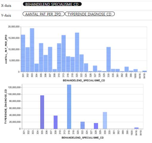
- We have looked at the Tableau-style PyGWalker app in Streamlit using the dataset bike_sharing_dc.csv. Other visualization examples include Airbnb EDA (implementing PyGWalker Dash UI in Jupyter IDE with gradio/NYC-Airbnb-Open-Data), the House price dataset from Kaggle to showcase the PyGWalker EDA in real estate, and PyGWalker EDA of Dutch eHealth Data .
- Image analysis: we have demonstrated the Keras Multi-Label Image Classification, Image Classification with ImageNet, Image-to-Sketch Conversion (converting RGB image to sketch using opencv library), BigGAN Text-to-Image, and Iris Flower Predictor pipelines and apps.
- ML Diabetes Prediction App: we have implemented the Diabetes Prediction App using the Gradio tutorial for ML (cf. Gradio documentation) and the SciKit-learn diabetes dataset. This includes the detailed RF Feature Engineering analysis involving partial dependence plots of selected model features.
- Super Soaker Failures Analysis demonstrated as the Gradio dashboard.
- The crop recommendation algorithm as multi-label classification (Decision Tree Classifier, Gaussian NB, SVM/SVC, Logistic Regression, and Random Forest Classifier) combined with Gradio deployment.
- We have employed the Hugging Face Transformers to perform NLP Sentiment Analysis as a pipeline.
- NLP sentence classification using the Persian demo model HooshvareLab/bert-fa-zwnj-base.
- LLM integration test: we have tried to generate our own D&D story using Opus MT and GPT-2.
- Article Summarization using the BeautifulSoup html parser and the default model sshleifer/distilbart-cnn-12-6 and revision a4f8f3e (https://huggingface.co/sshleifer/distilbart-cnn-12-6)
- Initializing EN-to-DE translation using t5-base and revision 686f1db (https://huggingface.co/t5-base) with the QC test.
- We have performed text substitution in Gradio, e.g. text.replace(‘World’, ‘Databricks’).
- We have implemented a simple app that predicts the score of a student based upon the number of study hours.
- We have examined story generation with GPT-2, BertForSequenceClassification, fill-mask, NER, and question answering.
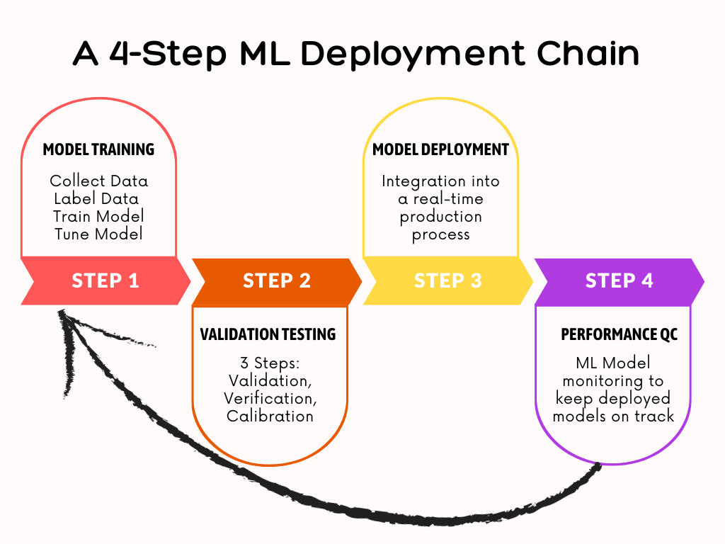
- While ML deployment is the third stage of the data science lifecycle (manage, develop, deploy and monitor), every aspect of a model’s creation is performed with deployment in mind. So final trained models can be accessed by end users.
- The Road Ahead: Implementing A 4-Step ML Deployment Chain (see below).
Explore More
- How to Deploy Machine Learning Models with Python & Streamlit
- Plotly Dash TA Stock Market App
- Low-Code AutoEDA of Dutch eHealth Data in Python
- An Implemented Streamlit Crop Prediction App
- Machine Learning-Based Crop Yield Prediction, Classification, and Recommendations
- Image Based Fast Forest Fire Detection with TensorFlow
- OpenAI’s ChatGPT VA Chatbots with/out Streamlit
- Advanced NLP Analysis & Stock Impact of ChatGPT-Related Tweets Q1’23
- An Interactive GPT Index and DeepLake Interface – 1. Amazon Financial Statements
- 90% ACC Diabetes-2 ML Binary Classifier
- AI-Driven Object Detection & Segmentation with Meta Detectron2 Deep Learning
- Multi-Label Keras CNN Image Classification of MNIST Fashion Clothing
- Case Study: Multi-Label Classification of Satellite Images with Fast.AI
- Comparative ML/AI Performance Analysis of 13 Handwritten Digit Recognition (HDR) Scikit-Learn Algorithms with PCA+HPO
- Semantic Analysis and NLP Visualizations of Wine Reviews
- ML/AI for Diabetes-2 Risk Management, Lifestyle/Daily-Life Support
- US Real Estate – Harnessing the Power of AI
- The Application of ML/AI in Diabetes
- A Comparison of ML/AI Diabetes-2 Binary Classification Algorithms
- 99% Accurate Breast Cancer Classification using Neural Networks in TensorFlow


Make a one-time donation
Make a monthly donation
Make a yearly donation
Choose an amount
Or enter a custom amount
Your contribution is appreciated.
Your contribution is appreciated.
Your contribution is appreciated.
DonateDonate monthlyDonate yearly
Leave a comment