- Nowadays, for professionals looking to build a career in data science, learning SQL is a must-have skill. Read more here.
- This all-inclusive SQL server tutorial helps data scientists get started with SQL straight away through many simple practical examples and exercises (with answers). The best way we learn SQL is by practice.
- The present tutorial also includes several important SQL basics cheat sheets, representing a quick guide to SQL commands and queries along with their examples and descriptions.
- In addition to numerous references and links to free online SQL resources, we have compiled a set of top SQL interview Q&A tailored to data scientists.
Become a SQL pro! Begin your SQL journey with confidence!
Table of Contents
- MS SQL Server Requirements
- RDBMS
- SQL SELECT Statement
- SQL Quieries with Constraints
- SQL ORDER BY Statement
- The SQL AND/OR Operator
- Multi-Table INNER JOIN Queries
- Multi-Table OUTER JOIN Queries
- SQL Queries with Expressions
- SQL Queries with Aggregates
- SQL Cheat Sheets
- Interview Q&A
- Discussion
- Conclusions
- The Road Ahead
- Resources
MS SQL Server Requirements
- For the sake of simplicity, we restrict ourselves to the MS SQL Server.
- MS SQL Server requires a minimum of 6 GB of available hard-disk space.
- Memory Express Editions: 1 GB.
- Processor Speed x64 Processor: 1.4 GHz
- Windows 10 TH1 1507 or greater with .NET Framework
- For more information on installing MS SQL Server on Server Core, see Install SQL Server on Server Core.
RDBMS
- RDBMS stands for Relational Database Management System.
- The data in RDBMS is stored in database objects called tables.
- A table is a data collection that consists of columns and rows (records).
- A field is a column in a table that is designed to maintain specific information about every record in the table (Customer ID, Address, City, etc.).
- A record is a horizontal entity in a table. A column is a vertical entity in a table that contains all information associated with a specific field in a table.
Example: Table Vehicles
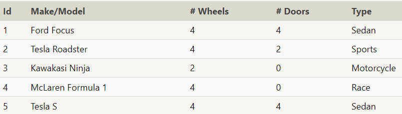
Key Takeaways:
- A relational database represents a collection of related (two-dimensional) tables.
- Each of the tables are similar to an Excel spreadsheet, with a fixed number of named columns (the attributes or properties of the table) and any number of rows of data.
SQL SELECT Statement
- The SELECT statement is used to query the database and retrieve selected data that match the criteria that you specify:
SELECT [ALL | DISTINCT] column1[,column2] FROM table1[,table2] [WHERE "conditions"] [GROUP BY "column-list"] [HAVING "conditions] [ORDER BY "column-list" [ASC | DESC] ]
- In the sequel, we will use the well-known Northwind sample database (aka Customers table):
Tablename	Records
Customers	91
Categories	8
Employees	10
OrderDetails	518
Orders	196
Products	77
Shippers	3
Suppliers	29
- Example:
- Return data from the Customers table
SELECT CustomerName,City FROM Customers;
- Result:
- Number of Records: 91

- Example: Select ALL columns
- Return all the columns from the Customers table
SELECT * FROM Customers;
- Result:
- Number of Records: 91

- For the sake of completeness, we will also be using a database with data about some of Pixar’s classic movies for most of our exercises. This exercise will involve the Movies table, and the default query below currently shows all the properties of each movie:
SELECT * FROM movies;
- Number of Records: 14
Table: Movies

- Find the
titleof each film
SELECT title FROM movies;

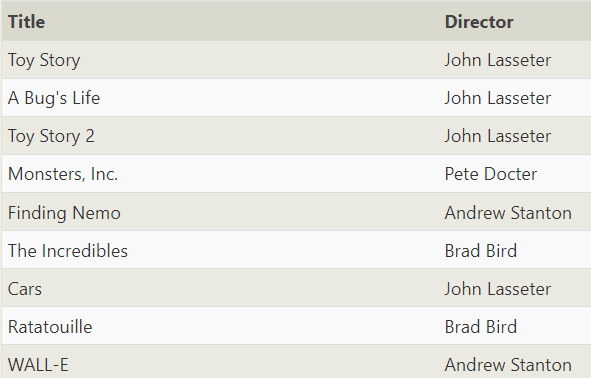
- Find the
directorof each film
SELECT director FROM movies;

- Find the
titleanddirectorof each film
SELECT title, director FROM movies;
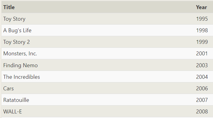
- Find the
titleandyearof each film
SELECT title, year FROM movies;
- Find
allthe information about each film
SELECT * FROM movies;
See Table Movies above.
SQL Quieries with Constraints
- Let’s apply the SQL WHERE Clause to the Customers table
SELECT * FROM Customers
WHERE Country='Mexico';
- Result Number of Records: 5

- Let’s look at the Movies table and find the movie with a row
idof 6
SELECT id, title FROM movies
WHERE id = 6;
- Output
| Id | Title |
| 6 | The Incredibles |
- Table Movies: Find the movies released in the
years between 2000 and 2010
SELECT title, year FROM movies
WHERE year BETWEEN 2000 AND 2010;
- Output
| Title | Year |
| Monsters, Inc. | 2001 |
| Finding Nemo | 2003 |
| The Incredibles | 2004 |
| Cars | 2006 |
| Ratatouille | 2007 |
| WALL-E | 2008 |
| Up | 2009 |
| Toy Story 3 | 2010 |
- Table Movies: Find the movies not released in the
years between 2000 and 2010
SELECT title, year FROM movies
WHERE year < 2000 OR year > 2010;
| Title | Year |
| Toy Story | 1995 |
| A Bug’s Life | 1998 |
| Toy Story 2 | 1999 |
| Cars 2 | 2011 |
| Brave | 2012 |
| Monsters University | 2013 |
- Table Movies: Find all the Toy Story movies
SELECT title, director FROM movies
WHERE title LIKE "Toy Story%";
| Title | Director |
| Toy Story | John Lasseter |
| Toy Story 2 | John Lasseter |
| Toy Story 3 | Lee Unkrich |
- Table Movies: Find all the movies directed by John Lasseter
SELECT title, director FROM movies
WHERE director = "John Lasseter";
| Title | Director |
| Toy Story | John Lasseter |
| A Bug’s Life | John Lasseter |
| Toy Story 2 | John Lasseter |
| Cars | John Lasseter |
| Cars 2 | John Lasseter |
- Table Movies: Find all the movies (and director) not directed by John Lasseter
SELECT title, director FROM movies
WHERE director != "John Lasseter";
| Title | Director |
| Monsters, Inc. | Pete Docter |
| Finding Nemo | Andrew Stanton |
| The Incredibles | Brad Bird |
| Ratatouille | Brad Bird |
| WALL-E | Andrew Stanton |
| Up | Pete Docter |
| Toy Story 3 | Lee Unkrich |
| Brave | Brenda Chapman |
| Monsters University | Dan Scanlon |
| WALL-G | Brenda Chapman |
- Table Movies: Find all the WALL-* movies
SELECT * FROM movies
WHERE title LIKE "WALL-_";
| Id | Title | Director | Year | Length_minutes |
| 9 | WALL-E | Andrew Stanton | 2008 | 104 |
| 87 | WALL-G | Brenda Chapman | 2042 | 97 |
- Table Movies: List all directors of Pixar movies (alphabetically), without duplicates
SELECT DISTINCT director FROM movies
ORDER BY director ASC;
| Director |
| Andrew Stanton |
| Brad Bird |
| Brenda Chapman |
| Dan Scanlon |
| John Lasseter |
| Lee Unkrich |
| Pete Docter |
SQL ORDER BY Statement
- Customers table: Sort the products by price
SELECT * FROM Products
ORDER BY Price;
- Result Number of Records: 77
| ProductID | ProductName | SupplierID | CategoryID | Unit | Price |
|---|---|---|---|---|---|
| 33 | Geitost | 15 | 4 | 500 g | 2.5 |
| 24 | Guaraná Fantástica | 10 | 1 | 12 – 355 ml cans | 4.5 |
| 13 | Konbu | 6 | 8 | 2 kg box | 6 |
| 52 | Filo Mix | 24 | 5 | 16 – 2 kg boxes | 7 |
| 54 | Tourtière | 25 | 6 | 16 pies | 7.45 |
| 75 | Rhönbräu Klosterbier | 12 | 1 | 24 – 0.5 l bottles | 7.75 |
| 23 | Tunnbröd | 9 | 5 | 12 – 250 g pkgs. | 9 |
| 19 | Teatime Chocolate Biscuits | 8 | 3 | 10 boxes x 12 pieces | 9.2 |
| 45 | Røgede sild | 21 | 8 | 1k pkg. | 9.5 |
| 47 | Zaanse koeken | 22 | 3 | 10 – 4 oz boxes | 9.5 |
| 41 | Jack’s New England Clam Chowder | 19 | 8 | 12 – 12 oz cans | 9.65 |
| 3 | Aniseed Syrup | 1 | 2 | 12 – 550 ml bottles | 10 |
- Customers table: Sort the products from highest to lowest price
SELECT * FROM Products
ORDER BY Price DESC;
- Result Number of Records: 77
| ProductID | ProductName | SupplierID | CategoryID | Unit | Price |
|---|---|---|---|---|---|
| 38 | Côte de Blaye | 18 | 1 | 12 – 75 cl bottles | 263.5 |
| 29 | Thüringer Rostbratwurst | 12 | 6 | 50 bags x 30 sausgs. | 123.79 |
| 9 | Mishi Kobe Niku | 4 | 6 | 18 – 500 g pkgs. | 97 |
| 20 | Sir Rodney’s Marmalade | 8 | 3 | 30 gift boxes | 81 |
| 18 | Carnarvon Tigers | 7 | 8 | 16 kg pkg. | 62.5 |
| 59 | Raclette Courdavault | 28 | 4 | 5 kg pkg. | 55 |
| 51 | Manjimup Dried Apples | 24 | 7 | 50 – 300 g pkgs. | 53 |
| 62 | Tarte au sucre | 29 | 3 | 48 pies | 49.3 |
| 43 | Ipoh Coffee | 20 | 1 | 16 – 500 g tins | 46 |
| 28 | Rössle Sauerkraut | 12 | 7 | 25 – 825 g cans | 45.6 |
| 27 | Schoggi Schokolade | 11 | 3 | 100 – 100 g pieces | 43.9 |
| 63 | Vegie-spread | 7 | 2 | 15 – 625 g jars | 43.9 |
| 8 | Northwoods Cranberry Sauce | 3 | 2 | 12 – 12 oz jars | 40 |
| 17 | Alice Mutton | 7 | 6 | 20 – 1 kg tins | 39 |
- Customers table: Sort the products alphabetically by Product Name
SELECT * FROM Products
ORDER BY ProductName;
- Result Number of Records: 77
| ProductID | ProductName | SupplierID | CategoryID | Unit | Price |
|---|---|---|---|---|---|
| 17 | Alice Mutton | 7 | 6 | 20 – 1 kg tins | 39 |
| 3 | Aniseed Syrup | 1 | 2 | 12 – 550 ml bottles | 10 |
| 40 | Boston Crab Meat | 19 | 8 | 24 – 4 oz tins | 18.4 |
| 60 | Camembert Pierrot | 28 | 4 | 15 – 300 g rounds | 34 |
| 18 | Carnarvon Tigers | 7 | 8 | 16 kg pkg. | 62.5 |
| 1 | Chais | 1 | 1 | 10 boxes x 20 bags | 18 |
| 2 | Chang | 1 | 1 | 24 – 12 oz bottles | 19 |
| 39 | Chartreuse verte | 18 | 1 | 750 cc per bottle | 18 |
| 4 | Chef Anton’s Cajun Seasoning | 2 | 2 | 48 – 6 oz jars | 22 |
| 5 | Chef Anton’s Gumbo Mix | 2 | 2 | 36 boxes | 21.35 |
| 48 | Chocolade | 22 | 3 | 10 pkgs. | 12.75 |
| 38 | Côte de Blaye | 18 | 1 | 12 – 75 cl bottles | 263.5 |
| 58 | Escargots de Bourgogne | 27 | 8 | 24 pieces | 13.25 |
- Select all customers from the Customers table, sorted ascending by the “Country” and descending by the “Customer Name” column
SELECT * FROM Customers
ORDER BY Country ASC, CustomerName DESC;
- Result Number of Records: 91
| CustomerID | CustomerName | ContactName | Address | City | PostalCode | Country |
|---|---|---|---|---|---|---|
| 64 | Rancho grande | Sergio Gutiérrez | Av. del Libertador 900 | Buenos Aires | 1010 | Argentina |
| 54 | Océano Atlántico Ltda. | Yvonne Moncada | Ing. Gustavo Moncada 8585 Piso 20-A | Buenos Aires | 1010 | Argentina |
| 12 | Cactus Comidas para llevar | Patricio Simpson | Cerrito 333 | Buenos Aires | 1010 | Argentina |
| 59 | Piccolo und mehr | Georg Pipps | Geislweg 14 | Salzburg | 5020 | Austria |
| 20 | Ernst Handel | Roland Mendel | Kirchgasse 6 | Graz | 8010 | Austria |
| 76 | Suprêmes délices | Pascale Cartrain | Boulevard Tirou, 255 | Charleroi | B-6000 | Belgium |
| 50 | Maison Dewey | Catherine Dewey | Rue Joseph-Bens 532 | Bruxelles | B-1180 | Belgium |
| 88 | Wellington Importadora | Paula Parente | Rua do Mercado, 12 | Resende | 08737-363 | Brazil |
| 81 | Tradição Hipermercados | Anabela Domingues | Av. Inês de Castro, 414 | São Paulo | 05634-030 | Brazil |
| 67 | Ricardo Adocicados | Janete Limeira | Av. Copacabana, 267 | Rio de Janeiro | 02389-890 | Brazil |
| 62 | Queen Cozinha | Lúcia Carvalho | Alameda dos Canàrios, 891 | São Paulo | 05487-020 | Brazil |
The SQL AND/OR Operator
- Customers table: Select all customers from Spain that starts with the letter ‘G’
SELECT * FROM Customers
WHERE Country = 'Spain' AND CustomerName LIKE 'G%';
- Result Number of Records: 2
| CustomerID | CustomerName | ContactName | Address | City | PostalCode | Country |
|---|---|---|---|---|---|---|
| 29 | Galería del gastrónomo | Eduardo Saavedra | Rambla de Cataluña, 23 | Barcelona | 08022 | Spain |
| 30 | Godos Cocina Típica | José Pedro Freyre | C/ Romero, 33 | Sevilla | 41101 | Spain |
- Customers table: Select all Spanish customers that starts with either “G” or “R”
SELECT * FROM Customers
WHERE Country = 'Spain'
AND (CustomerName LIKE 'G%' OR CustomerName LIKE 'R%');
- Result Number of Records: 3
| CustomerID | CustomerName | ContactName | Address | City | PostalCode | Country |
|---|---|---|---|---|---|---|
| 29 | Galería del gastrónomo | Eduardo Saavedra | Rambla de Cataluña, 23 | Barcelona | 08022 | Spain |
| 30 | Godos Cocina Típica | José Pedro Freyre | C/ Romero, 33 | Sevilla | 41101 | Spain |
| 69 | Romero y tomillo | Alejandra Camino | Gran Vía, 1 | Madrid | 28001 | Spain |
- Customers table: Select all customers from Germany or Spain
SELECT *
FROM Customers
WHERE Country = 'Germany' OR Country = 'Spain';
- Result Number of Records: 16
| CustomerID | CustomerName | ContactName | Address | City | PostalCode | Country |
|---|---|---|---|---|---|---|
| 1 | Alfreds Futterkiste | Maria Anders | Obere Str. 57 | Berlin | 12209 | Germany |
| 6 | Blauer See Delikatessen | Hanna Moos | Forsterstr. 57 | Mannheim | 68306 | Germany |
| 8 | Bólido Comidas preparadas | Martín Sommer | C/ Araquil, 67 | Madrid | 28023 | Spain |
| 17 | Drachenblut Delikatessend | Sven Ottlieb | Walserweg 21 | Aachen | 52066 | Germany |
| 22 | FISSA Fabrica Inter. Salchichas S.A. | Diego Roel | C/ Moralzarzal, 86 | Madrid | 28034 | Spain |
| 25 | Frankenversand | Peter Franken | Berliner Platz 43 | München | 80805 | Germany |
| 29 | Galería del gastrónomo | Eduardo Saavedra | Rambla de Cataluña, 23 | Barcelona | 08022 | Spain |
| 30 | Godos Cocina Típica | José Pedro Freyre | C/ Romero, 33 | Sevilla | 41101 | Spain |
| 39 | Königlich Essen | Philip Cramer | Maubelstr. 90 | Brandenburg | 14776 | Germany |
| 44 | Lehmanns Marktstand | Renate Messner | Magazinweg 7 | Frankfurt a.M. | 60528 | Germany |
| 52 | Morgenstern Gesundkost | Alexander Feuer | Heerstr. 22 | Leipzig | 04179 | Germany |
| 56 | Ottilies Käseladen | Henriette Pfalzheim | Mehrheimerstr. 369 | Köln | 50739 | Germany |
| 63 | QUICK-Stop | Horst Kloss | Taucherstraße 10 | Cunewalde | 01307 | Germany |
| 69 | Romero y tomillo | Alejandra Camino | Gran Vía, 1 | Madrid | 28001 | Spain |
| 79 | Toms Spezialitäten | Karin Josephs | Luisenstr. 48 | Münster | 44087 | Germany |
| 86 | Die Wandernde Kuh | Rita Müller | Adenauerallee 900 | Stuttgart | 70563 | Germany |
Multi-Table INNER JOIN Queries
- Table: Movies
| Id | Title | Director | Year | Length_minutes |
| 1 | Toy Story | John Lasseter | 1995 | 81 |
| 2 | A Bug’s Life | John Lasseter | 1998 | 95 |
| 3 | Toy Story 2 | John Lasseter | 1999 | 93 |
| 4 | Monsters, Inc. | Pete Docter | 2001 | 92 |
| 5 | Finding Nemo | Andrew Stanton | 2003 | 107 |
| 6 | The Incredibles | Brad Bird | 2004 | 116 |
| 7 | Cars | John Lasseter | 2006 | 117 |
| 8 | Ratatouille | Brad Bird | 2007 | 115 |
| 9 | WALL-E | Andrew Stanton | 2008 | 104 |
| 10 | Up | Pete Docter | 2009 | 101 |
| 11 | Toy Story 3 | Lee Unkrich | 2010 | 103 |
| 12 | Cars 2 | John Lasseter | 2011 | 120 |
| 13 | Brave | Brenda Chapman | 2012 | 102 |
| 14 | Monsters University | Dan Scanlon | 2013 | 110 |
- Table: Box-office
| Movie_id | Rating | Domestic_sales | International_sales |
| 5 | 8.2 | 380843261 | 555900000 |
| 14 | 7.4 | 268492764 | 475066843 |
| 8 | 8 | 206445654 | 417277164 |
| 12 | 6.4 | 191452396 | 368400000 |
| 3 | 7.9 | 245852179 | 239163000 |
| 6 | 8 | 261441092 | 370001000 |
| 9 | 8.5 | 223808164 | 297503696 |
| 11 | 8.4 | 415004880 | 648167031 |
| 1 | 8.3 | 191796233 | 170162503 |
| 7 | 7.2 | 244082982 | 217900167 |
| 10 | 8.3 | 293004164 | 438338580 |
| 4 | 8.1 | 289916256 | 272900000 |
| 2 | 7.2 | 162798565 | 200600000 |
| 13 | 7.2 | 237283207 | 301700000 |
- Find the domestic and international sales for each movie
SELECT title, domestic_sales, international_sales
FROM movies
  JOIN boxoffice
    ON movies.id = boxoffice.movie_id;
| Title | Domestic_sales | International_sales |
| Finding Nemo | 380843261 | 555900000 |
| Monsters University | 268492764 | 475066843 |
| Ratatouille | 206445654 | 417277164 |
| Cars 2 | 191452396 | 368400000 |
| Toy Story 2 | 245852179 | 239163000 |
| The Incredibles | 261441092 | 370001000 |
| WALL-E | 223808164 | 297503696 |
| Toy Story 3 | 415004880 | 648167031 |
| Toy Story | 191796233 | 170162503 |
| Cars | 244082982 | 217900167 |
| Up | 293004164 | 438338580 |
| Monsters, Inc. | 289916256 | 272900000 |
| A Bug’s Life | 162798565 | 200600000 |
| Brave | 237283207 | 301700000 |
- Show the sales numbers for each movie that did better internationally rather than domestically
SELECT title, domestic_sales, international_sales
FROM movies
  JOIN boxoffice
    ON movies.id = boxoffice.movie_id
WHERE international_sales > domestic_sales;
| Title | Domestic_sales | International_sales |
| Finding Nemo | 380843261 | 555900000 |
| Monsters University | 268492764 | 475066843 |
| Ratatouille | 206445654 | 417277164 |
| Cars 2 | 191452396 | 368400000 |
| The Incredibles | 261441092 | 370001000 |
| WALL-E | 223808164 | 297503696 |
| Toy Story 3 | 415004880 | 648167031 |
| Up | 293004164 | 438338580 |
| A Bug’s Life | 162798565 | 200600000 |
| Brave | 237283207 | 301700000 |
- List all the movies by their ratings in descending order
SELECT title, rating
FROM movies
  JOIN boxoffice
    ON movies.id = boxoffice.movie_id
ORDER BY rating DESC;
| Title | Rating |
| WALL-E | 8.5 |
| Toy Story 3 | 8.4 |
| Toy Story | 8.3 |
| Up | 8.3 |
| Finding Nemo | 8.2 |
| Monsters, Inc. | 8.1 |
| Ratatouille | 8 |
| The Incredibles | 8 |
| Toy Story 2 | 7.9 |
| Monsters University | 7.4 |
| Cars | 7.2 |
| A Bug’s Life | 7.2 |
| Brave | 7.2 |
| Cars 2 | 6.4 |
Multi-Table OUTER JOIN Queries
- Table Buildings
| Building_name | Capacity |
| 1e | 24 |
| 1w | 32 |
| 2e | 16 |
| 2w | 20 |
- Table Employees
| Role | Name | Building | Years_employed |
| Engineer | Becky A. | 1e | 4 |
| Engineer | Dan B. | 1e | 2 |
| Engineer | Sharon F. | 1e | 6 |
| Engineer | Dan M. | 1e | 4 |
| Engineer | Malcom S. | 1e | 1 |
| Artist | Tylar S. | 2w | 2 |
| Artist | Sherman D. | 2w | 8 |
| Artist | Jakob J. | 2w | 6 |
| Artist | Lillia A. | 2w | 7 |
| Artist | Brandon J. | 2w | 7 |
| Manager | Scott K. | 1e | 9 |
| Manager | Shirlee M. | 1e | 3 |
| Manager | Daria O. | 2w | 6 |
- Find the list of all buildings that have employees
SELECT DISTINCT building FROM employees;
| Building |
| 1e |
| 2w |
- Find the list of all buildings and their capacity
SELECT * FROM buildings;
| Building_name | Capacity |
| 1e | 24 |
| 1w | 32 |
| 2e | 16 |
| 2w | 20 |
- List all buildings and the distinct employee roles in each building (including empty buildings)
SELECT DISTINCT building_name, role
FROM buildings
  LEFT JOIN employees
    ON building_name = building;
| Building_name | Role |
| 1e | Engineer |
| 1e | Manager |
| 1w | |
| 2e | |
| 2w | Artist |
| 2w | Manager |
SQL Queries with Expressions
- We are going to have to use expressions to transform the Box Office table into something easier
- Input data
Table Movies
| Id | Title | Director | Year | Length_minutes |
| 1 | Toy Story | John Lasseter | 1995 | 81 |
| 2 | A Bug’s Life | John Lasseter | 1998 | 95 |
| 3 | Toy Story 2 | John Lasseter | 1999 | 93 |
| 4 | Monsters, Inc. | Pete Docter | 2001 | 92 |
| 5 | Finding Nemo | Andrew Stanton | 2003 | 107 |
| 6 | The Incredibles | Brad Bird | 2004 | 116 |
| 7 | Cars | John Lasseter | 2006 | 117 |
| 8 | Ratatouille | Brad Bird | 2007 | 115 |
| 9 | WALL-E | Andrew Stanton | 2008 | 104 |
| 10 | Up | Pete Docter | 2009 | 101 |
| 11 | Toy Story 3 | Lee Unkrich | 2010 | 103 |
| 12 | Cars 2 | John Lasseter | 2011 | 120 |
| 13 | Brave | Brenda Chapman | 2012 | 102 |
| 14 | Monsters University | Dan Scanlon | 2013 | 110 |
Table Box Office
| Movie_id | Rating | Domestic_sales | International_sales |
| 5 | 8.2 | 380843261 | 555900000 |
| 14 | 7.4 | 268492764 | 475066843 |
| 8 | 8 | 206445654 | 417277164 |
| 12 | 6.4 | 191452396 | 368400000 |
| 3 | 7.9 | 245852179 | 239163000 |
| 6 | 8 | 261441092 | 370001000 |
| 9 | 8.5 | 223808164 | 297503696 |
| 11 | 8.4 | 415004880 | 648167031 |
| 1 | 8.3 | 191796233 | 170162503 |
| 7 | 7.2 | 244082982 | 217900167 |
| 10 | 8.3 | 293004164 | 438338580 |
| 4 | 8.1 | 289916256 | 272900000 |
| 2 | 7.2 | 162798565 | 200600000 |
| 13 | 7.2 | 237283207 | 301700000 |
- List all movies and their combined sales in millions of dollars
SELECT title, (domestic_sales + international_sales) / 1000000 AS gross_sales_millions
FROM movies
  JOIN boxoffice
    ON movies.id = boxoffice.movie_id;
Query Results:
| Title | Gross_sales_millions |
| Finding Nemo | 936.743261 |
| Monsters University | 743.559607 |
| Ratatouille | 623.722818 |
| Cars 2 | 559.852396 |
| Toy Story 2 | 485.015179 |
| The Incredibles | 631.442092 |
| WALL-E | 521.31186 |
| Toy Story 3 | 1063.171911 |
| Toy Story | 361.958736 |
| Cars | 461.983149 |
| Up | 731.342744 |
| Monsters, Inc. | 562.816256 |
| A Bug’s Life | 363.398565 |
| Brave | 538.983207 |
- List all movies and their ratings in percent
SELECT title, rating * 10 AS rating_percent
FROM movies
  JOIN boxoffice
    ON movies.id = boxoffice.movie_id;
Query Results
| Title | Rating_percent |
| Finding Nemo | 82 |
| Monsters University | 74 |
| Ratatouille | 80 |
| Cars 2 | 64 |
| Toy Story 2 | 79 |
| The Incredibles | 80 |
| WALL-E | 85 |
| Toy Story 3 | 84 |
| Toy Story | 83 |
| Cars | 72 |
| Up | 83 |
| Monsters, Inc. | 81 |
| A Bug’s Life | 72 |
| Brave | 72 |
- List all movies that were released on even number years
SELECT title, year
FROM movies
WHERE year % 2 = 0;
Query Results
| Title | Year |
| A Bug’s Life | 1998 |
| The Incredibles | 2004 |
| Cars | 2006 |
| WALL-E | 2008 |
| Toy Story 3 | 2010 |
| Brave | 2012 |
SQL Queries with Aggregates
- SQL also supports the use of aggregate expressions (or functions) that allow you to summarize information about a group of rows of data.
- Table: Employees
| Role | Name | Building | Years_employed |
| Engineer | Becky A. | 1e | 4 |
| Engineer | Dan B. | 1e | 2 |
| Engineer | Sharon F. | 1e | 6 |
| Engineer | Dan M. | 1e | 4 |
| Engineer | Malcom S. | 1e | 1 |
| Artist | Tylar S. | 2w | 2 |
| Artist | Sherman D. | 2w | 8 |
| Artist | Jakob J. | 2w | 6 |
| Artist | Lillia A. | 2w | 7 |
| Artist | Brandon J. | 2w | 7 |
| Manager | Scott K. | 1e | 9 |
| Manager | Shirlee M. | 1e | 3 |
| Manager | Daria O. | 2w | 6 |
- Find the longest time that an employee has been at the studio
SELECT MAX(years_employed) as Max_years_employed
FROM employees;
Output:
| Max_years_employed |
| 9 |
- For each role, find the average number of years employed by employees in that role
SELECT role, AVG(years_employed) as Average_years_employed
FROM employees
GROUP BY role;
Output:
| Role | Average_years_employed |
| Artist | 6 |
| Engineer | 3.4 |
| Manager | 6 |
- Find the total number of employee years worked in each building
SELECT building, SUM(years_employed) as Total_years_employed
FROM employees
GROUP BY building;
| Building | Total_years_employed |
| 1e | 29 |
| 2w | 36 |
Read more here.
SQL Cheat Sheets
| Command | Syntax | Description |
| SELECT | SELECT column, another column, … FROM mytable; | The result of this query will be a two-dimensional set of rows and columns, effectively a copy of the table, but only with the columns that we requested. |
| WHERE | SELECT column, another_column, … FROM mytable WHERE condition AND/OR another_condition AND/OR …; | The clause is applied to each row of data by checking specific column values to determine whether it should be included in the results or not. |
| DISTINCT | SELECT DISTINCT column, another_column, … FROM mytable WHERE condition(s); | The clause provides a convenient way to discard rows that have a duplicate column value |
| ORDER BY | SELECT column, another_column, … FROM mytable WHERE condition(s) ORDER BY column ASC/DESC; | The clause provides a way to sort your results by a given column in ascending or descending order |
LIMIT and OFFSET | SELECT column, another_column, … FROM mytable WHERE condition(s) ORDER BY column ASC/DESC LIMIT num_limit OFFSET num_offset; | The LIMIT will reduce the number of rows to return, and the optional OFFSET will specify where to begin counting the number rows from. |
| INNER JOIN | SELECT column, another_table_column, … FROM mytable INNER JOIN another_table ON mytable.id = another_table.id WHERE condition(s) ORDER BY column, … ASC/DESC LIMIT num_limit OFFSET num_offset; | The INNER JOIN is a process that matches rows from the first table and the second table which have the same key (as defined by the ON constraint) to create a result row with the combined columns from both tables. |
| OUTER JOINs | SELECT column, another_column, … FROM mytable INNER/LEFT/RIGHT/FULL JOIN another_table ON mytable.id = another_table.matching_id WHERE condition(s) ORDER BY column, … ASC/DESC LIMIT num_limit OFFSET num_offset; | When joining table A to table B, a LEFT JOIN simply includes rows from A regardless of whether a matching row is found in B. The RIGHT JOIN is the same, but reversed, keeping rows in B regardless of whether a match is found in A. Finally, a FULL JOIN simply means that rows from both tables are kept, regardless of whether a matching row exists in the other table. |
| NULL | SELECT column, another_column, … FROM mytable WHERE column IS/IS NOT NULL AND/OR another_condition AND/OR …; | If your database needs to store incomplete data, then NULL values can be appropriate, especially when the default values will skew later analysis. |
| Queries with expressions | SELECT col_expression AS expr_description, … FROM mytable; | Use them in the SELECT part of the query, and give them descriptive alias using the AS keyword. |
| Queries with aggregates | SELECT AGG_FUNC(column_or_expression) AS aggregate_description, … FROM mytable WHERE constraint_expression GROUP BY column; | SQL also supports the use of aggregate expressions (or functions) that allow you to summarize information about a group of rows of data. |
Read more here.
Interview Q&A
| Question | Answer |
| What are the five basic SQL commands? | ALTER, UPDATE, DELETE, INSERT, and CREATE |
| How are SQL commands classified? | Data Definition Language (DDL) Data Manipulation Language (DML) Data Control Language (DCL) Transaction Control Language (TCL) Data Query Language (DQL) |
| How do you create/delete a table in SQL? | CREATE TABLEDROP TABLE |
| What are constraints in SQL? | Constraints are the rules that are set for the data that can be placed inside a table: NOT NULL: The data in this column cannot include any null values. UNIQUE: Every entry in this column needs to be unique. PRIMARY KEY: These are columns that have data that are unique for each record in the column. CHECK: This constraint checks every entry in a column for a specific condition. FOREIGN KEY: These are columns with attributes that refer to the primary key of a different table. DEFAULT: This constraint sets a default value for when no value is entered. CREATE INDEX: This is used to create indexes in tables so that data can be retrieved quickly. |
| How do you change a table name in SQL? | RENAME old new |
| How do you delete a row in SQL? | DELETE FROM Cars WHERE sno=6 |
| How do you create a database in SQL? | CREATE DATABASE StudentInfo |
| Define an index, along with its different types | An index is a table that has two columns. The first column is a duplicate of the primary key of a table. The second column has pointers to where the key value of each record is stored. Primary index (dense index and sparse index) Secondary index Clustering index Multi-level index B-tree index |
| What is PL/SQL? | PL/SQL is short for Procedural Language Extensions to the Structured Query Language. It gives software developers a way to combine SQL with procedural statements like the ones used in general-purpose programming languages. |
| What is MySQL? | MySQL is an open-source relational database management system software. It was created by Oracle and based on SQL. |
| What are the different types of relationships in SQL? | There are three main types of relationships between data values in SQL. They are: One-to-one relationship: This implies that a record in the first table is related to only one record in the second table. One-to-many relationship: In a one-to-many relationship, a record in the first table can be related to one or more records in the second table. But the records in the second table can be related only to one record in the first table. Many-to-many relationship: In this kind of relationship, multiple records in the first table are related to multiple records in the second table. |
| What is a schema in SQL? | A schema is a logical representation of the different objects in the database. Think of it as a mapping of all the tables, functions, stored procedures, and indexes that are part of a database. |
| Discuss standard clauses used with SELECT query in SQL? | WHERE: Used to select items based on a specific set of conditions GROUP BY: Used to group rows whose values match that of the result set ORDER BY: Arranges the resulting set in descending or ascending order TOP: Sets a limit on the number of records returned by a query HAVING: Serves the same function as the WHERE clause except that it can be used with aggregate functions |
| Explain UNION, MINUS, and INTERSECT commands. | The UNION command combines the output of two select queries into a single result. INTERSECT is also a binary set operator like the UNION command, except that it outputs the rows that are in common between the results of two SELECT queries. The MINUS command is the opposite of the INTERSECT command. When you apply MINUS to the results of two SELECT queries, it returns the rows that are in the first selection but not in the second one. |
| What is a “view” in SQL? | A view is a table that holds data from one or multiple tables in an SQL database, but doesn’t actually physically exist in the memory. |
| How to use BETWEEN in SQL? | The BETWEEN statement in SQL is used to select values that fall within a particular range. These values can be text, numbers, or dates. |
| What is the difference between an inner join and an outer join? | An inner join focuses on the data that two tables have in common. It is essentially the intersection of the two datasets. An outer join also includes the data that two tables have in common. But along with that, it also returns rows for which there is no match in the other table. |
| What is the difference between B-Tree and hash indexing in SQL? | Balanced trees, or B-trees, are used to make comparisons between columns that use the =, >, >=, <, <= operators or the BETWEEN clause. Hash indexes are used for comparisons using only the operators = or ⇔. |
| What is the difference between UNION and UNION ALL? | The difference between the UNION and UNION ALL commands lies in the way they treat duplicate records. When you use the UNION command, it combines the data in two tables, but also eliminates duplicate data. UNION ALL doesn’t remove duplicate values and combines all of the data in the two tables. |
| How and when do you use the GROUP BY function? | The GROUP BY command quite simply groups rows in a table that have the same values. |
| What are the most common aggregate functions in SQL? | COUNT – Counts the number of rows in a specific table or a view AVG – Calculates the average value from a given set of values MAX – Identifies the maximum value in a given set of values MIN – Identifies the minimum value in a given set of values SUM – Outputs the sum of a given set of values |
| How do you copy a table in SQL? | SELECT * INTO T2 FROM T1; |
| What is the SQL Injection? | SQL injection is a code injection technique that might destroy your database. SQL injection is one of the most common web hacking techniques. SQL injection is the placement of malicious code in SQL statements, via web page input. |
| What are SQL editors? | With online SQL editors, you can edit SQL statements, and view the result in your browser. |
| What is PostgreSQL? | PostgreSQL is an open-source relational database system with advanced features for enterprise use cases. It offers support for most of the popular programming languages, including Python, C, Javascript, Java, and Ruby. |
| What is a trigger in SQL? | A trigger is a specialized procedure in SQL which runs automatically when a particular event occurs or a certain condition has been met. |
| What are the differences between SQL and Transact Structured Query Language (TSQL)? | SQL was developed by IBM whereas TSQL was developed by Microsoft. SQL is used to execute one query at a time to insert, update, or delete the data in a database. TSQL makes it possible to carry out transactional activities in a database using various programmatic techniques. SQL is focused on manipulating the data in a database. TSQL is used to build applications and implement business logic within them. |
| What are the differences between MongoDB and SQL? | SQL databases are relational in nature whereas MongoDB has non-relational databases. SQL uses the commands and statements in the SQL query language. MongoDB uses JSON as its query language. SQL is vertically scalable, whereas MongoDB is horizontally scalable. SQL focuses on the properties of ACID: atomicity, consistency, isolation, and durability. MongoDB emphasizes CAP properties: consistency, availability, and partition tolerance. |
| What are the differences between NoSQL and SQL? | SQL is a database management software that supports the storage and analysis of structured data. NoSQL allows you to store and retrieve structured data but also offers support for unstructured and polymorphic data. SQL was created in the year 1970 to deal with problems relating to file storage. NoSQL came about in the early 2000s as a way to allow databases to handle semi-structured and unstructured data. SQL is vertically scalable, which means that you can add resources so that the existing hardware and software can handle greater capacities. NoSQL is horizontally scalable and lets you add larger nodes to smaller nodes to enhance its capacity. There is no support for storing data hierarchically in SQL whereas NoSQL is especially suited to handling hierarchical data. SQL doesn’t support the distribution of data, which means that one installation can only run on one system. Features like partition and repetition mean that NoSQL allows data distribution. |
Read more here.
Discussion
- Let’s discuss SQL using Python, viz. integrating SQLite3 with Python
- To use SQLite, we must import sqlite3
- Then create a connection using connect() method and pass the name of the database
- After this, a cursor object is called to be capable to send commands to the SQL
- Output: Connected to the database
- To execute a query in the database, create an object and write the SQL command in it with being commented. Example:- sql_comm = ”SQL statement”
- Execute the command: call the cursor method execute() and pass the name of the sql command as a parameter in it.
Conclusions
- SQL (Structured Query Language) is a language to operate databases
- SQL is an ANSI/ISO certified standard and mostly all the RDMS like MySQL, MS Access, Oracle, Sybase, Informix, PostgreSQL and SQL Server use SQL as a standard database query language
- SQL is a medium to communicate with the data stored in the relational database. It can perform all the CRUD (CREATE, RETRIEVE, UPDATE, DELETE) operations in the database
- SQL is used by most of the database programs present. (i.e. SQL Server, MYSQL, SQLite, etc.)
- SQL is widely popular because it offers the following advantages:
- Allows users to access data in the relational database management systems.
- Allows users to describe the data.
- Allows users to define the data in a database and manipulate that data.
- Allows to embed within other languages using SQL modules, libraries & pre-compilers.
- Allows users to create and drop databases and tables.
- Allows users to create view, stored procedure, functions in a database.
- Allows users to set permissions on tables, procedures and views.
The Road Ahead
10 Advanced SQL Concepts You Should Know for Data Science Interviews:
- Common table expressions (CTEs).
- Recursive CTEs.
- Temporary functions.
- Pivoting data with case when.
- Except versus Not In.
- Self joins.
- Rank versus dense rank versus row number.
- Calculating delta values.
- Calculating running totals.
- Date-time manipulation.
Resources
- w3schools, w3resource
- SQL Practice 1
- sqbolt
- 9 Websites you can practice SQL for FREE
- 7 Best Platforms to Practice SQL
- 17 Sites for SQL Practice
- The best & quickest way to learn SQL
- How can I practice SQL at home for free?
- Want to learn and master PL/SQL?
- Learn and share SQL
- SQL Interview Questions
- MS SQL Training
- SQL Interview Questions and Answers
- 105 SQL Interview Questions
- Basic SQL Guide


One-Time
Monthly
Yearly
Make a one-time donation
Make a monthly donation
Make a yearly donation
Choose an amount
€5.00
€15.00
€100.00
€5.00
€15.00
€100.00
€5.00
€15.00
€100.00
Or enter a custom amount
€
Your contribution is appreciated.
Your contribution is appreciated.
Your contribution is appreciated.
DonateDonate monthlyDonate yearly
Leave a comment