Top 6 Reliability/Risk Engineering Learnings

Featured Photo by Kammeran Gonzalez-Keola on Pexels

Today we will review and test the Eric Marsden’s e-learning Python courseware and training materials on risk engineering, loss prevention and safety management under the Terms & Conditions of the Creative Commons Attribution-ShareAlike license.

Table of Contents

1. Lifetime of Light Bulbs
2. Failure of Electronic Components
3. Maintenance of a Large Computing Facility
4. Failure of Pumps in an Oil Field
5. Stock Value at Risk (VaR)
6. Stock Correlations
7. Summary
8. Explore More

Lifetime of Light Bulbs

Input: The lifetime of a light bulb is known to be exponentially distributed with a mean of 5000 hours.

• Q1. Find the proportion of bulbs that may be expected to fail before 4000 hours of use.
• Q2 What is the lifetime that we have 95% confidence will be exceeded?

Solution:

import numpy
import scipy.stats

dist = scipy.stats.expon(scale=5000)
dist.cdf(4000)

0.5506710358827784

The result Q2 is expressed in hours
dist.ppf(0.05)

256.46647193775266

Q1: So about 55% of light bulbs will fail before they reach 4000 hours of operation.

Q2: The 0.05 quantile of the lifetime distribution is 256 hours.

Read More about Survival Analysis.

Failure of Electronic Components

Input: An electronic device will function if both components function correctly. The lifetimes of the 1st and the 2nd components is known to be exponentially distributed with a mean of 3000 and 5000 hours, respectively.

Task: Find the proportion of devices that may be expected to fail before 4000 hours use.

Solution:

The probability of the 1st component still working after 4000 hours is

pa = 1 – scipy.stats.expon(scale=3000).cdf(4000)
pa

0.2635971381157267

and likewise for the 2nd component

pb = 1 – scipy.stats.expon(scale=5000).cdf(4000)
pb

0.44932896411722156

The probability of both working is

pa * pb

0.11844182901380367

So, the proportion of devices that can be expected to fail before 4000 hours’ use is around 88%.

Maintenance of a Large Computing Facility

Input (the maintenance logbook)

15 downtimes over 1 month, 1200 min in emergency maintenance

Tasks:

• The MTTR (mean time to repair) and repair rate
• The probability that the warranty requirement <100 min is being met
• The median time to repair
• The time within which 95% of the maintenance actions can be completed.

Solution:

• MTTR = 1200/15 = 80 min

• The repair rate = 1/MTTR = 1/80 = 0.0125
• PPD of repair time is

dist = scipy.stats.expon(scale=80)

• The probability of time to repair < 100 min is

dist.cdf(100)

0.7134952031398099

• The median time to repair = 0.5 quantile (min)

dist.ppf(0.5)

55.451774444795625

• The time (min) of 95% completed maintenance

dist.ppf(0.95)

239.6585818843192

Failure of Pumps in an Oil Field

Input

From field data in an oil field, the time to failure of a pump, X, is known to be normally distributed. The mean and standard deviation of the time to failure are estimated from historical data as 3200 and 600 hours, respectively.

Task

• What is the probability that a pump X will fail after it has worked for 2000 h?
• If 2 pumps work in parallel, what is probability that the system will fail after it has worked for 2000 h?

Solution

• The probability P(X<2000) = 1 – P(X>2000)

1 – scipy.stats.norm(3200, 600).cdf(2000)

0.9772498680518208

That is the probability of the system working for at least 2000 h is 1 – that of both pumps failing before 2000 hours, which is 1 – 0.977², or 0.9994.

• Given that pump failure is independent, that’s 1 – P(X1<2000) *P(X2<2000)

1 – scipy.stats.norm(3200, 600).cdf(2000)**2

0.9994824314963404

Stock Value at Risk (VaR)

Let’s look at stock market trends and Value at Risk (VaR).

We begin by setting the working directory RISK

import os
os.chdir(‘RISK’)
os. getcwd()

• Importing libraries

import numpy

import pandas

import scipy.stats

import matplotlib.pyplot as plt

from yahoofinancials import YahooFinancials
from datetime import datetime

plt.style.use(“bmh”)

%config InlineBackend.figure_formats=[“png”]

• Introducing the function

def retrieve_stock_data(ticker, start, end):
json = YahooFinancials(ticker).get_historical_price_data(start, end, “daily”)
df = pandas.DataFrame(columns=[“open”,”close”,”adjclose”])
for row in json[ticker][“prices”]:
date = datetime.fromisoformat(row[“formatted_date”])
df.loc[date] = [row[“open”], row[“close”], row[“adjclose”]]
df.index.name = “date”
return df

• Reading the $MO stock data

MSFT = retrieve_stock_data(“MO”, “2021-01-01”, “2023-04-02”)
fig = plt.figure()
fig.set_size_inches(10,3)
MSFT[“adjclose”].plot()
plt.title(“MO Stock”, weight=”bold”);
plt.savefig(‘mostockprice.png’)

• Let’s calculate the MO daily returns

• Let’s plot the histogram of MO daily returns and calculate std

MSFT[“adjclose”].pct_change().hist(bins=50, density=True, histtype=”stepfilled”, alpha=0.5)
plt.title(“Histogram of MO daily returns”, weight=”bold”)
MSFT[“adjclose”].pct_change().std()

0.014316580881876793

• Let’s look at the Q-Q normal distribution plot

Q = MSFT[“adjclose”].pct_change().dropna()
scipy.stats.probplot(Q, dist=scipy.stats.norm, plot=plt.figure().add_subplot(111))
plt.title(“Normal probability plot of MO daily returns”, weight=”bold”);

• Similarly, we can plot the MO Student-t distribution Q-Q plot

tdf, tmean, tsigma = scipy.stats.t.fit(Q)
scipy.stats.probplot(Q, dist=scipy.stats.t, sparams=(tdf, tmean, tsigma), plot=plt.figure().add_subplot(111))
plt.title(“Student probability plot of MO daily returns”, weight=”bold”);

• Let’s look at the rival stock PM in terms of VaR using the historical bootstrap method. We begin with the PM daily returns

stock = retrieve_stock_data(“PM”, “2021-01-01”, “2023-04-02”)
returns = stock[“adjclose”].pct_change().dropna()
mean = returns.mean()
sigma = returns.std()
tdf, tmean, tsigma = scipy.stats.t.fit(returns)
returns.hist(bins=40, density=True, histtype=”stepfilled”, alpha=0.5)
plt.title(“PM daily returns”, weight=”bold”);

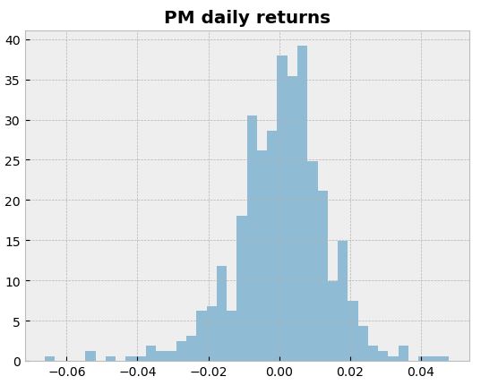
returns.quantile(0.05)

-0.021812384359857478

The 0.05 empirical quantile of daily returns is at -0.02. That means that with 95% confidence, our worst daily loss will not exceed 2%. If we have a 1 M€ investment, our one-day 5% VaR is 0.02 * 1 M€ = 20 k€.

• Let’s check VaR using the variance-covariance method

support = numpy.linspace(returns.min(), returns.max(), 100)
returns.hist(bins=40, density=True, histtype=”stepfilled”, alpha=0.5);
plt.plot(support, scipy.stats.t.pdf(support, loc=tmean, scale=tsigma, df=tdf), “r-“)
plt.title(“PM Daily change (%)”, weight=”bold”);

scipy.stats.norm.ppf(0.05, mean, sigma)

-0.021253176229908726

• VaR using the Monte Carlo method

Let’s define the parameters of the geometric Brownian motion

days = 300 # time horizon
dt = 1/float(days)
sigma = 0.04 # volatility
mu = 0.05 # drift (average growth rate)

• Let’s define the random walk function

def random_walk(startprice):
price = numpy.zeros(days)
shock = numpy.zeros(days)
price[0] = startprice
for i in range(1, days):
shock[i] = numpy.random.normal(loc=mu * dt, scale=sigma * numpy.sqrt(dt))
price[i] = max(0, price[i-1] + shock[i] * price[i-1])
return price

• Let’s simulate 30 random walks, starting from an initial stock price of 10€, for a duration of 300 days

plt.figure(figsize=(9,4))
for run in range(30):
plt.plot(random_walk(10.0))
plt.xlabel(“Time”)
plt.ylabel(“Price”);

Final price is spread out between 9.5€ (our portfolio has lost value) to almost 11.25€. We can see graphically that the expectation (mean outcome) is a profit; this is due to the fact that the drift in our random walk (parameter mu) is positive.

• Now let’s run a big Monte Carlo simulation of random walks of this type, to obtain the probability distribution of the final price, and obtain quantile measures for the VaR estimation

runs = 10000
simulations = numpy.zeros(runs)
for run in range(runs):
simulations[run] = random_walk(10.0)[days-1]
q = numpy.percentile(simulations, 1)
plt.hist(simulations, density=True, bins=30, histtype=”stepfilled”, alpha=0.5)
plt.figtext(0.6, 0.8, “Start price: 10€”)
plt.figtext(0.6, 0.7, “Mean final price: {:.3}€”.format(simulations.mean()))
plt.figtext(0.6, 0.6, “VaR(0.99): {:.3}€”.format(10 – q))
plt.figtext(0.15, 0.6, “q(0.99): {:.3}€”.format(q))
plt.axvline(x=q, linewidth=4, color=”r”)
plt.title(“Final price distribution after {} days”.format(days), weight=”bold”);

We have looked at the 1% empirical quantile of the final PM price distribution to estimate VaR, which is 0.431€ for a 10€ investment.

Stock Correlations

Let’s compare the variation of different stock indexes: CAC40 (France), DAX (Germany), the Hang Seng Index in Hong Kong, and the All Ordinaries in Australia:

start = “2021-01-01”
end = “2023-04-02”
CAC = retrieve_stock_data(“^FCHI”, start, end)
DAX = retrieve_stock_data(“^GDAXI”, start, end)
HSI = retrieve_stock_data(“^HSI”, start, end)
AORD = retrieve_stock_data(“^AORD”, start, end)

df = pandas.DataFrame({ “CAC”: CAC[“adjclose”].pct_change(),
“DAX”: DAX[“adjclose”].pct_change(),
“HSI”: HSI[“adjclose”].pct_change(),
“AORD”: AORD[“adjclose”].pct_change() })
dfna = df.dropna()

ax = plt.axes()
ax.set_xlim(-0.15, 0.15)
ax.set_ylim(-0.15, 0.15)
plt.plot(dfna[“CAC”], dfna[“DAX”], “r.”, alpha=0.5)
plt.xlabel(“CAC40 daily return”)
plt.ylabel(“DAX daily return”)
plt.title(“CAC vs DAX daily returns”, weight=”bold”);

scipy.stats.pearsonr(dfna[“CAC”], dfna[“DAX”])

PearsonRResult(statistic=0.9311647843546521, pvalue=2.4314191441635316e-213)

This is a high level of correlation between the French and German indexes. 

• Let’s examine AORD vs CAC

ax = plt.axes()
ax.set_xlim(-0.15, 0.15)
ax.set_ylim(-0.15, 0.15)
plt.plot(dfna[“CAC”], dfna[“AORD”], “r.”, alpha=0.5)
plt.xlabel(“CAC40 daily return”)
plt.ylabel(“All Ordinaries daily return”)
plt.title(“CAC vs All Ordinaries index daily returns”, weight=”bold”);

scipy.stats.pearsonr(dfna[“CAC”], dfna[“AORD”])

PearsonRResult(statistic=0.32833306998596323, pvalue=1.2526560187261144e-13)

Here the level of correlation is much lower: daily returns of French and Australian firms are fairly different.

• Let’s check the CAC t-fit

returns = dfna[“CAC”]
returns.hist(bins=30, density=True, histtype=”stepfilled”, alpha=0.5)
support = numpy.linspace(returns.min(), returns.max(), 100)
tdf, tmean, tsigma = scipy.stats.t.fit(returns)
print(“CAC t fit: mean={}, scale={}, df={}”.format(tmean, tsigma, tdf))
plt.plot(support, scipy.stats.t.pdf(support, loc=tmean, scale=tsigma, df=tdf), “r-“)
plt.figtext(0.6, 0.7, “tμ = {:.3}”.format(tmean))
plt.figtext(0.6, 0.65, “tσ = {:.3}”.format(tsigma))
plt.figtext(0.6, 0.6, “df = {:.3}”.format(tdf))
plt.title(“Histogram of CAC40 daily returns”, weight=”bold”);

CAC t fit: mean=0.001179259800176915, scale=0.008089826249985525, df=4.079039153491818

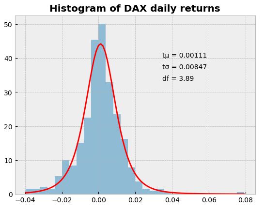
• Similarly, we can check the DAX t-fit

returns = dfna[“DAX”]
returns.hist(bins=30, density=True, histtype=”stepfilled”, alpha=0.5)
support = numpy.linspace(returns.min(), returns.max(), 100)
tdf, tmean, tsigma = scipy.stats.t.fit(returns)
print(“DAX t fit: mean={}, scale={}, df={}”.format(tmean, tsigma, tdf))
plt.plot(support, scipy.stats.t.pdf(support, loc=tmean, scale=tsigma, df=tdf), “r-“)
plt.figtext(0.6, 0.7, “tμ = {:.3}”.format(tmean))
plt.figtext(0.6, 0.65, “tσ = {:.3}”.format(tsigma))
plt.figtext(0.6, 0.6, “df = {:.3}”.format(tdf))
plt.title(“Histogram of DAX daily returns”, weight=”bold”);

DAX t fit: mean=0.0011149895731915964, scale=0.00846914354053661, df=3.889032152342769

Summary

• We discussed top 6 learning examples related to risk engineering, loss prevention and safety management. 

• Industrial applications of risk engineering include health and safety in the oil and gas sector, nuclear energy, chemicals manufacturing, aviation, railways, civil engineering and critical infrastructure management.
• We also looked at market risk used in the finance, banking and insurance industries. We estimated VaR using statistical simulations, while analyzing the effect of portfolio diversification and correlation between stocks on financial risk.

Explore More

• Risk Engineering
• Applying a Risk-Aware Portfolio Rebalancing Strategy to ETF, Energy, Pharma, and Aerospace/Defense Stocks in 2023
• Towards Max(ROI/Risk) Trading in Q1 2023
• Stock Portfolio Risk/Return Optimization
• Risk/Return QC via Portfolio Optimization – Current Positions of The Dividend Breeder
• Investment Risk Management Study

---