
Featured Photo by cottonbro studio, Pexels
Facial Recognition (FR) is a category of biometric software that maps an individual’s facial features mathematically and stores the data as a faceprint.
The goal of this case study is the Exploratory Data Analysis (EDA) and performance QC analysis of out-of-box ML/AI workflows tested on public-domain datasets and real-time webcam GUI.
Table of Contents
The Face Dataset
In the field of FR, SVM has been shown to be superior to other techniques in terms of accuracy and robustness. SVM works well with small datasets, and it is also able to handle complex patterns and noisy data. This makes it an ideal algorithm for FR.
First, we need to import the FR data. The Scikit-Learn library provides inbuilt face recognition datasets including the popular one, the LFW (Labelled Faces in The Wild) dataset. This dataset consists of around 14000 labeled images with each having a label associated with it. These images are of human faces and they have been manually annotated by researchers from around the world.
Let’s set the working directory YOURPATH
import os
os.chdir(‘YOURPATH’)
os. getcwd()
and import the LFW dataset
from sklearn.datasets import fetch_lfw_people
faces = fetch_lfw_people(min_faces_per_person=60)
with the description
faces.DESCR
(see Appendix).
Let’s plot some of the faces using the matplotlib imshow method
import matplotlib.pyplot as plt
fig, splts = plt.subplots(2, 4)
for i, splts in enumerate(splts.flat):
splts.imshow(faces.images[i])
splts.set(xticks=[], yticks=[],
xlabel=faces.target_names[faces.target[i]])
plt.savefig(‘inputfacesbush.png’)

Splitting the dataset using train_test_split with test_size=0.2
from sklearn.model_selection import train_test_split
X = faces.data
y = faces.target
X_train, X_test, y_train, y_test = train_test_split(X, y, test_size=0.2, random_state=42)
X_train.shape
(1078, 2914)
X_test.shape
(270, 2914)
Let’s import SVC and RandomizedPCA from sklearn
from sklearn.svm import SVC
from sklearn.decomposition import PCA as RandomizedPCA
from sklearn.pipeline import make_pipeline
For dimensionality reduction
pca = RandomizedPCA(n_components=150, whiten=True, random_state=42)
svc = SVC(kernel=’rbf’, class_weight=’balanced’)
model = make_pipeline(pca, svc)
Let’s train our model using the above ML pipeline
model.fit(X_train, y_train)

Testing the model:
from sklearn.metrics import accuracy_score
predictions = model.predict(X_test)
accuracy_score(predictions, y_test)
0.762962962962963
Let’s compare erroneous predictions made by the model and actual values
from colorama import Fore
incorrect = 0
length = len(predictions)
print(“Actual\t\t\t\tPredicted\n”)
for i in range(len(predictions)):
if predictions[i] != y_test[i]: # if predictions and actual values are not equal
prediction_name = faces.target_names[predictions[predictions[i]]] # Getting the predicted name
actual_name = faces.target_names[y_test[y_test[i]]] # Getting the actual name
incorrect+=1
print(“{}\t\t\t{}”.format(Fore.GREEN + actual_name, Fore.RED+prediction_name))
print(“{} are classified as correct and {} are classified as incorrect!”.format(length-incorrect, incorrect))
Actual				Predicted

Junichiro Koizumi			George W Bush
Junichiro Koizumi			George W Bush
Gerhard Schroeder			Junichiro Koizumi
George W Bush			Tony Blair
George W Bush			Junichiro Koizumi
Colin Powell			Junichiro Koizumi
George W Bush			Junichiro Koizumi
George W Bush			Junichiro Koizumi
Junichiro Koizumi			George W Bush
George W Bush			Junichiro Koizumi
Colin Powell			Tony Blair
George W Bush			George W Bush
Colin Powell			Junichiro Koizumi
George W Bush			Junichiro Koizumi
George W Bush			Junichiro Koizumi
Junichiro Koizumi			George W Bush
Colin Powell			Junichiro Koizumi
Junichiro Koizumi			Junichiro Koizumi
Gerhard Schroeder			George W Bush
Gerhard Schroeder			Junichiro Koizumi
Junichiro Koizumi			George W Bush
Gerhard Schroeder			George W Bush
George W Bush			Tony Blair
Junichiro Koizumi			Junichiro Koizumi
George W Bush			Tony Blair
George W Bush			Junichiro Koizumi
George W Bush			George W Bush
George W Bush			Junichiro Koizumi
George W Bush			Junichiro Koizumi
George W Bush			Junichiro Koizumi
Colin Powell			George W Bush
George W Bush			Junichiro Koizumi
George W Bush			George W Bush
George W Bush			Junichiro Koizumi
George W Bush			Junichiro Koizumi
Colin Powell			Junichiro Koizumi
Colin Powell			Junichiro Koizumi
George W Bush			Junichiro Koizumi
Gerhard Schroeder			Junichiro Koizumi
Gerhard Schroeder			Junichiro Koizumi
Junichiro Koizumi			Tony Blair
Gerhard Schroeder			Junichiro Koizumi
George W Bush			Junichiro Koizumi
George W Bush			Junichiro Koizumi
Gerhard Schroeder			George W Bush
Gerhard Schroeder			Junichiro Koizumi
Junichiro Koizumi			Tony Blair
George W Bush			Junichiro Koizumi
Junichiro Koizumi			George W Bush
Colin Powell			Junichiro Koizumi
George W Bush			Tony Blair
George W Bush			Tony Blair
Junichiro Koizumi			Tony Blair
George W Bush			Junichiro Koizumi
Junichiro Koizumi			George W Bush
George W Bush			Junichiro Koizumi
Junichiro Koizumi			Junichiro Koizumi
Junichiro Koizumi			Tony Blair
Junichiro Koizumi			Junichiro Koizumi
Colin Powell			Tony Blair
Junichiro Koizumi			George W Bush
George W Bush			Junichiro Koizumi
Junichiro Koizumi			George W Bush
George W Bush			Tony Blair
206 are classified as correct and 64 are classified as incorrect!
Let’s look at the classification report
from sklearn.metrics import classification_report
print(classification_report(predictions, y_test, digits=2))
precision    recall  f1-score   support

           0       0.58      0.78      0.67         9
           1       0.82      0.81      0.82        52
           2       0.60      0.83      0.70        18
           3       0.92      0.73      0.81       124
           4       0.57      0.86      0.69        14
           5       0.40      1.00      0.57         6
           6       0.80      0.89      0.84         9
           7       0.68      0.68      0.68        38

    accuracy                           0.76       270
   macro avg       0.67      0.82      0.72       270
weighted avg       0.80      0.76      0.77       270
Let’s examine the confusion matrix
from sklearn.metrics import confusion_matrix
matrix = confusion_matrix(predictions, y_test)
matrix
array([[ 7,  0,  1,  1,  0,  0,  0,  0],
       [ 1, 42,  1,  3,  0,  2,  0,  3],
       [ 0,  1, 15,  0,  1,  0,  0,  1],
       [ 4,  6,  6, 90,  4,  4,  2,  8],
       [ 0,  0,  0,  0, 12,  2,  0,  0],
       [ 0,  0,  0,  0,  0,  6,  0,  0],
       [ 0,  0,  0,  0,  1,  0,  8,  0],
       [ 0,  2,  2,  4,  3,  1,  0, 26]], dtype=int64)
Let’s plot this matrix as the seaborn heatmap
import seaborn as sns
from sklearn import metrics
import numpy as np # linear algebra
import pandas as pd # data processing, CSV file I/O (e.g. pd.read_csv)
plt.figure(1, figsize=(12,8))
cm = metrics.confusion_matrix(predictions, y_test)
cmn = cm.astype(‘float’) / cm.sum(axis=1)[:, np.newaxis]
sns.heatmap(cmn,cmap=’Blues’,annot=True)
plt.ylabel(‘Actual’)
plt.xlabel(‘Predicted’)
plt.title(‘SVC Normalized Confusion Matrix’)
plt.savefig(‘pcasvcconfusionmatrixbushblair.png’)
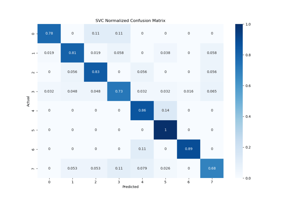
Recall that a perfect classifier has a confusion matrix in which all the values are zero except diagonals.
The Olivetti Dataset
Next, let’s apply FR to the Kaggle Olivetti dataset:
- Face images taken between April 1992 and April 1994.
- There are ten different image of each of 40 distinct people
- There are 400 face images in the dataset
- Face images were taken at different times, variying ligthing, facial express and facial detail
- All face images have black background
- The images are gray level
- Size of each image is 64×64
- Image pixel values were scaled to [0, 1] interval
- Names of 40 people were encoded to an integer from 0 to 39.
Let’s import and/or install the key libraries
!pip install mglearn
import numpy as np # linear algebra
import pandas as pd # data processing, CSV file I/O (e.g. pd.read_csv)
Visualization
import matplotlib.pyplot as plt
Machine Learning
from sklearn.model_selection import train_test_split
from sklearn.decomposition import PCA
from sklearn.svm import SVC
from sklearn.naive_bayes import GaussianNB
from sklearn.neighbors import KNeighborsClassifier
from sklearn.tree import DecisionTreeClassifier
from sklearn.linear_model import LogisticRegression
from sklearn.discriminant_analysis import LinearDiscriminantAnalysis
from sklearn import metrics
import warnings
warnings.filterwarnings(‘ignore’)
print(“Warnings ignored!!”)
import mglearn
Warnings ignored!!
Let’s read the input data and print info
data=np.load(“olivetti_faces.npy”)
target=np.load(“olivetti_faces_target.npy”)
print(“There are {} images in the dataset”.format(len(data)))
print(“There are {} unique targets in the dataset”.format(len(np.unique(target))))
print(“Size of each image is {}x{}”.format(data.shape[1],data.shape[2]))
print(“Pixel values were scaled to [0,1] interval. e.g:{}”.format(data[0][0,:4]))
There are 400 images in the dataset
There are 40 unique targets in the dataset
Size of each image is 64x64
Pixel values were scaled to [0,1] interval. e.g:[0.30991736 0.3677686  0.41735536 0.44214877]
print(“unique target number:”,np.unique(target))
unique target number: [ 0  1  2  3  4  5  6  7  8  9 10 11 12 13 14 15 16 17 18 19 20 21 22 23
 24 25 26 27 28 29 30 31 32 33 34 35 36 37 38 39]
data.shape
(400, 64, 64)
target.shape
(400,)
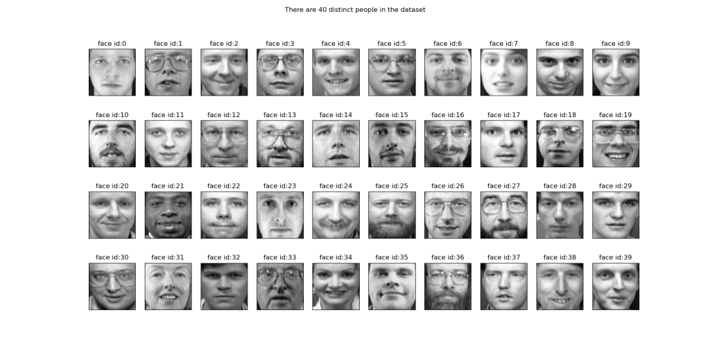
Let’s look at images of 40 Distinct People in the Olivetti Dataset
def show_40_distinct_people(images, unique_ids):
#Creating 4X10 subplots in 18×9 figure size
fig, axarr=plt.subplots(nrows=4, ncols=10, figsize=(18, 9))
#For easy iteration flattened 4X10 subplots matrix to 40 array
axarr=axarr.flatten()
#iterating over user ids
for unique_id in unique_ids:
    image_index=unique_id*10
    axarr[unique_id].imshow(images[image_index], cmap='gray')
    axarr[unique_id].set_xticks([])
    axarr[unique_id].set_yticks([])
    axarr[unique_id].set_title("face id:{}".format(unique_id))
plt.suptitle("There are 40 distinct people in the dataset")
plt.savefig('40_distinct_people.png')
show_40_distinct_people(data, np.unique(target))
We can also see other people faces by selecting different values of subject_ids
show_10_faces_of_n_subject(images=data, subject_ids=[2,7, 23, 26, 38])
![People faces with subject_ids=[2,7, 23, 26, 38]](https://newdigitals.org/wp-content/uploads/2023/03/10_faces_of_n_subject.png?w=1024)
show_10_faces_of_n_subject(images=data, subject_ids=[0,5, 21, 24, 36])

Let’s reshape images for our ML model
X=data.reshape((data.shape[0],data.shape[1]*data.shape[2]))
print(“X shape:”,X.shape)
X=data.reshape((data.shape[0],data.shape[1]*data.shape[2]))
print(“X shape:”,X.shape)
X shape: (400, 4096)
Let’s apply train_test_split with test_size=0.2
X_train, X_test, y_train, y_test=train_test_split(X, target, test_size=0.2, stratify=target, random_state=0)
print(“X_train shape:”,X_train.shape)
print(“y_train shape:{}”.format(y_train.shape))
X_train shape: (320, 4096)
y_train shape:(320,)
Let’s check the number of y-data samples per target class
y_frame=pd.DataFrame()
y_frame[‘subject ids’]=y_train
y_frame.groupby([‘subject ids’]).size().plot.bar(figsize=(15,8),title=”Number of Samples per Target Class”)
plt.savefig(‘numberofsamples.png’)

Principal Component Analysis (PCA) is the unsupervised ML technique that allows to reduce the dimension of the data by selecting the most important components. Let’s illustrate PCA with a simple synthetic 2D test
mglearn.plots.plot_pca_illustration()
plt.savefig(‘pca_illustration.png’)

The algorithm proceeds by finding the direction of the maximum variance labeled “Component 1”.
Let’s implement PCA as follows
from sklearn.decomposition import PCA
pca=PCA(n_components=2)
pca.fit(X)
X_pca=pca.transform(X)
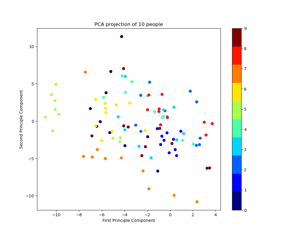
Let’s plot the 2D PCA projection of 10 people
number_of_people=10
index_range=number_of_people*10
fig=plt.figure(figsize=(10,8))
ax=fig.add_subplot(1,1,1)
scatter=ax.scatter(X_pca[:index_range,0],
X_pca[:index_range,1],
c=target[:index_range],
s=40,
cmap=plt.get_cmap(‘jet’, number_of_people)
)
ax.set_xlabel(“First Principle Component”)
ax.set_ylabel(“Second Principle Component”)
ax.set_title(“PCA projection of {} people”.format(number_of_people))
fig.colorbar(scatter)
plt.savefig(‘pcaprojection10people.png’)
Let’s check the PCA explained variances vs components
pca=PCA()
pca.fit(X)
plt.figure(1, figsize=(12,8))
plt.plot(pca.explained_variance_, linewidth=2)
plt.xlabel(‘Components’)
plt.ylabel(‘Explained Variaces’)
plt.savefig(‘pcaexplainedvariances.png’)
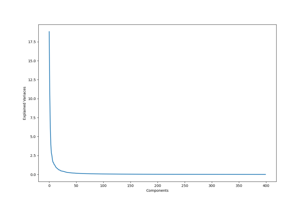
Let’s apply PCA with n_components=90 as the Optimum Number of principal components
n_components=90
pca=PCA(n_components=n_components, whiten=True)
pca.fit(X_train)
PCA(n_components=90, whiten=True)
We can apply PCA with svd_solver
PCA(copy=True, iterated_power=’auto’, n_components=90, random_state=None,
svd_solver=’auto’, tol=0.0, whiten=True)
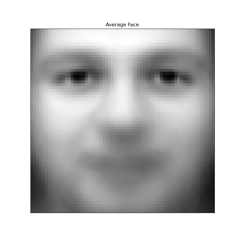
and plot the low-resolution average face
fig,ax=plt.subplots(1,1,figsize=(8,8))
ax.imshow(pca.mean_.reshape((64,64)), cmap=”gray”)
ax.set_xticks([])
ax.set_yticks([])
ax.set_title(‘Average Face’)
plt.savefig(‘averageface.png’)
We can also plot all face eigenimages
number_of_eigenfaces=len(pca.components_)
eigen_faces=pca.components_.reshape((number_of_eigenfaces, data.shape[1], data.shape[2]))
cols=10
rows=int(number_of_eigenfaces/cols)
fig, axarr=plt.subplots(nrows=rows, ncols=cols, figsize=(15,15))
axarr=axarr.flatten()
for i in range(number_of_eigenfaces):
axarr[i].imshow(eigen_faces[i],cmap=”gray”)
axarr[i].set_xticks([])
axarr[i].set_yticks([])
axarr[i].set_title(“eigen id:{}”.format(i))
plt.suptitle(“All Eigen Faces”.format(10“=”, 10“=”))
plt.savefig(‘alleigenfaces.png’)

Let’s apply PCA to both train and test data
X_train_pca=pca.transform(X_train)
X_test_pca=pca.transform(X_test)
Let’s apply the SVC kernel to the PCA-transformed train/test data
clf = SVC()
clf.fit(X_train_pca, y_train)
y_pred = clf.predict(X_test_pca)
print(“accuracy score:{:.2f}”.format(metrics.accuracy_score(y_test, y_pred)))
accuracy score:0.94
print(metrics.f1_score(y_test, y_pred,average=’macro’))
0.9349999999999999
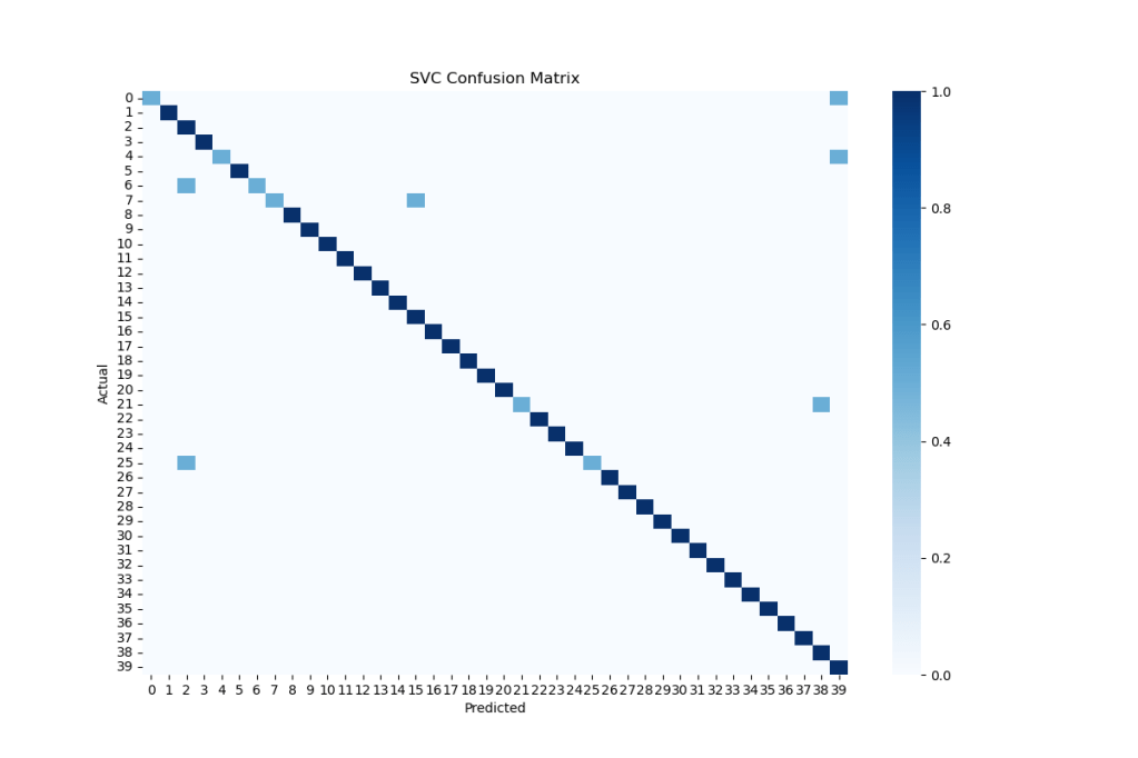
Let’s plot the SVC confusion matrix as the seaborn heatmap
import seaborn as sns
plt.figure(1, figsize=(12,8))
cm = metrics.confusion_matrix(y_test, y_pred)
cmn = cm.astype(‘float’) / cm.sum(axis=1)[:, np.newaxis]
sns.heatmap(cmn,annot=False,cmap=’Blues’)
plt.ylabel(‘Actual’)
plt.xlabel(‘Predicted’)
plt.xlabel(‘SVC Confusion Matrix’)
plt.savefig(‘confusionmatrixblue.png’)
Let’s print the classification report
print(metrics.classification_report(y_test, y_pred))
precision    recall  f1-score   support

           0       1.00      0.50      0.67         2
           1       1.00      1.00      1.00         2
           2       0.50      1.00      0.67         2
           3       1.00      1.00      1.00         2
           4       1.00      0.50      0.67         2
           5       1.00      1.00      1.00         2
           6       1.00      0.50      0.67         2
           7       1.00      0.50      0.67         2
           8       1.00      1.00      1.00         2
           9       1.00      1.00      1.00         2
          10       1.00      1.00      1.00         2
          11       1.00      1.00      1.00         2
          12       1.00      1.00      1.00         2
          13       1.00      1.00      1.00         2
          14       1.00      1.00      1.00         2
          15       0.67      1.00      0.80         2
          16       1.00      1.00      1.00         2
          17       1.00      1.00      1.00         2
          18       1.00      1.00      1.00         2
          19       1.00      1.00      1.00         2
          20       1.00      1.00      1.00         2
          21       1.00      0.50      0.67         2
          22       1.00      1.00      1.00         2
          23       1.00      1.00      1.00         2
          24       1.00      1.00      1.00         2
          25       1.00      0.50      0.67         2
          26       1.00      1.00      1.00         2
          27       1.00      1.00      1.00         2
          28       1.00      1.00      1.00         2
          29       1.00      1.00      1.00         2
          30       1.00      1.00      1.00         2
          31       1.00      1.00      1.00         2
          32       1.00      1.00      1.00         2
          33       1.00      1.00      1.00         2
          34       1.00      1.00      1.00         2
          35       1.00      1.00      1.00         2
          36       1.00      1.00      1.00         2
          37       1.00      1.00      1.00         2
          38       0.67      1.00      0.80         2
          39       0.50      1.00      0.67         2

    accuracy                           0.93        80
   macro avg       0.96      0.93      0.92        80
weighted avg       0.96      0.93      0.92        80
Let’s compare several ML classifiers
from sklearn.linear_model import SGDClassifier
from sklearn.ensemble import RandomForestClassifier
models=[]
models.append((‘LDA’, LinearDiscriminantAnalysis()))
models.append((“LR”,LogisticRegression()))
models.append((“NB”,GaussianNB()))
models.append((“KNN”,KNeighborsClassifier(n_neighbors=5)))
models.append((“DT”,DecisionTreeClassifier()))
models.append((“SVM”,SVC()))
models.append((“SGD”,SGDClassifier()))
models.append((‘RF’, RandomForestClassifier()))
for name, model in models:
clf=model

clf.fit(X_train_pca, y_train)

y_pred=clf.predict(X_test_pca)
print(10*"=","{} Result".format(name).upper(),10*"=")
print("Accuracy score:{:0.2f}".format(metrics.accuracy_score(y_test, y_pred)))
print()
========== LDA RESULT ==========
Accuracy score:0.95

========== LR RESULT ==========
Accuracy score:0.94

========== NB RESULT ==========
Accuracy score:0.91

========== KNN RESULT ==========
Accuracy score:0.75

========== DT RESULT ==========
Accuracy score:0.60

========== SVM RESULT ==========
Accuracy score:0.93

========== SGD RESULT ==========
Accuracy score:0.93

========== RF RESULT ==========
Accuracy score:0.94
Let’s check cross_val_score
from sklearn.model_selection import cross_val_score
from sklearn.model_selection import KFold
pca=PCA(n_components=n_components, whiten=True)
pca.fit(X)
X_pca=pca.transform(X)
for name, model in models:
kfold=KFold(n_splits=5, shuffle=True, random_state=0)
cv_scores=cross_val_score(model, X_pca, target, cv=kfold)
print("{} mean cross validations score:{:.2f}".format(name, cv_scores.mean()))
LDA mean cross validations score:0.97
LR mean cross validations score:0.94
NB mean cross validations score:0.80
KNN mean cross validations score:0.70
DT mean cross validations score:0.50
SVM mean cross validations score:0.88
SGD mean cross validations score:0.91
RF mean cross validations score:0.89
Let’s examine the LDA classifier
lr=LinearDiscriminantAnalysis()
lr.fit(X_train_pca, y_train)
y_pred=lr.predict(X_test_pca)
print(“Accuracy score:{:.2f}”.format(metrics.accuracy_score(y_test, y_pred)))
Accuracy score:0.96
Let’s plot the LDA Confusion Matrix
import seaborn as sns
plt.figure(1, figsize=(12,8))
cm = metrics.confusion_matrix(y_test, y_pred)
cmn = cm.astype(‘float’) / cm.sum(axis=1)[:, np.newaxis]
sns.heatmap(cmn,annot=False,cmap=’Blues’)
plt.ylabel(‘Actual’)
plt.xlabel(‘Predicted’)
plt.title(‘LDA Confusion Matrix’)
plt.savefig(‘ldconfusionmatrixblue.png’)

Let’s print the LDA classification report
print(“Classification Results:\n{}”.format(metrics.classification_report(y_test, y_pred)))
Classification Results:
              precision    recall  f1-score   support

           0       1.00      1.00      1.00         2
           1       1.00      1.00      1.00         2
           2       0.67      1.00      0.80         2
           3       1.00      1.00      1.00         2
           4       1.00      0.50      0.67         2
           5       1.00      1.00      1.00         2
           6       1.00      1.00      1.00         2
           7       1.00      0.50      0.67         2
           8       1.00      1.00      1.00         2
           9       1.00      1.00      1.00         2
          10       1.00      1.00      1.00         2
          11       1.00      1.00      1.00         2
          12       1.00      1.00      1.00         2
          13       1.00      1.00      1.00         2
          14       1.00      1.00      1.00         2
          15       1.00      1.00      1.00         2
          16       1.00      1.00      1.00         2
          17       1.00      1.00      1.00         2
          18       1.00      1.00      1.00         2
          19       1.00      1.00      1.00         2
          20       1.00      1.00      1.00         2
          21       1.00      0.50      0.67         2
          22       1.00      1.00      1.00         2
          23       1.00      1.00      1.00         2
          24       1.00      1.00      1.00         2
          25       1.00      1.00      1.00         2
          26       1.00      1.00      1.00         2
          27       1.00      1.00      1.00         2
          28       1.00      1.00      1.00         2
          29       1.00      1.00      1.00         2
          30       1.00      1.00      1.00         2
          31       1.00      1.00      1.00         2
          32       1.00      1.00      1.00         2
          33       1.00      1.00      1.00         2
          34       1.00      1.00      1.00         2
          35       1.00      1.00      1.00         2
          36       1.00      1.00      1.00         2
          37       1.00      1.00      1.00         2
          38       0.67      1.00      0.80         2
          39       0.67      1.00      0.80         2

    accuracy                           0.96        80
   macro avg       0.97      0.96      0.96        80
weighted avg       0.97      0.96      0.96        80
Let’s run various ML optimization scenarios:
- LogisticRegression + LeaveOneOut
from sklearn.model_selection import LeaveOneOut
loo_cv=LeaveOneOut()
clf=LogisticRegression()
cv_scores=cross_val_score(clf,
X_pca,
target,
cv=loo_cv)
print(“{} Leave One Out cross-validation mean accuracy score:{:.2f}”.format(clf.class.name,
cv_scores.mean()))
LogisticRegression Leave One Out cross-validation mean accuracy score:0.96
- LDA + LeaveOneOut
from sklearn.model_selection import LeaveOneOut
loo_cv=LeaveOneOut()
clf=LinearDiscriminantAnalysis()
cv_scores=cross_val_score(clf,
X_pca,
target,
cv=loo_cv)
print(“{} Leave One Out cross-validation mean accuracy score:{:.2f}”.format(clf.class.name,
cv_scores.mean()))
LinearDiscriminantAnalysis Leave One Out cross-validation mean accuracy score:0.98
- Hyperparameter Tuning: GridSearcCV
from sklearn.model_selection import GridSearchCV
from sklearn.model_selection import LeaveOneOut
params={‘penalty’:[‘l1’, ‘l2’],
‘C’:np.logspace(0, 4, 10)
}
clf=LogisticRegression()
loo_cv=LeaveOneOut()
gridSearchCV=GridSearchCV(clf, params, cv=loo_cv)
gridSearchCV.fit(X_train_pca, y_train)
print(“Grid search fitted..”)
print(gridSearchCV.best_params_)
print(gridSearchCV.best_score_)
print(“grid search cross validation score:{:.2f}”.format(gridSearchCV.score(X_test_pca, y_test)))
Grid search fitted..
{'C': 1.0, 'penalty': 'l2'}
0.934375
grid search cross validation score:0.94
- LR + PCA + OneVsRestClassifier
lr=LogisticRegression(C=1.0, penalty=”l2″)
lr.fit(X_train_pca, y_train)
print(“lr score:{:.2f}”.format(lr.score(X_test_pca, y_test)))
lr score:0.94
from sklearn.preprocessing import label_binarize
from sklearn.multiclass import OneVsRestClassifier
Target=label_binarize(target, classes=range(40))
print(Target.shape)
print(Target[0])
n_classes=Target.shape[1]
(400, 40)
[1 0 0 0 0 0 0 0 0 0 0 0 0 0 0 0 0 0 0 0 0 0 0 0 0 0 0 0 0 0 0 0 0 0 0 0 0
 0 0 0]
Splitting multi-class data
X_train_multiclass, X_test_multiclass, y_train_multiclass, y_test_multiclass=train_test_split(X, Target, test_size=0.2,
stratify=Target, random_state=0)
pca=PCA(n_components=n_components, whiten=True)
pca.fit(X_train_multiclass)
X_train_multiclass_pca=pca.transform(X_train_multiclass)
X_test_multiclass_pca=pca.transform(X_test_multiclass)
oneRestClassifier=OneVsRestClassifier(lr)
oneRestClassifier.fit(X_train_multiclass_pca, y_train_multiclass)
y_score=oneRestClassifier.decision_function(X_test_multiclass_pca)
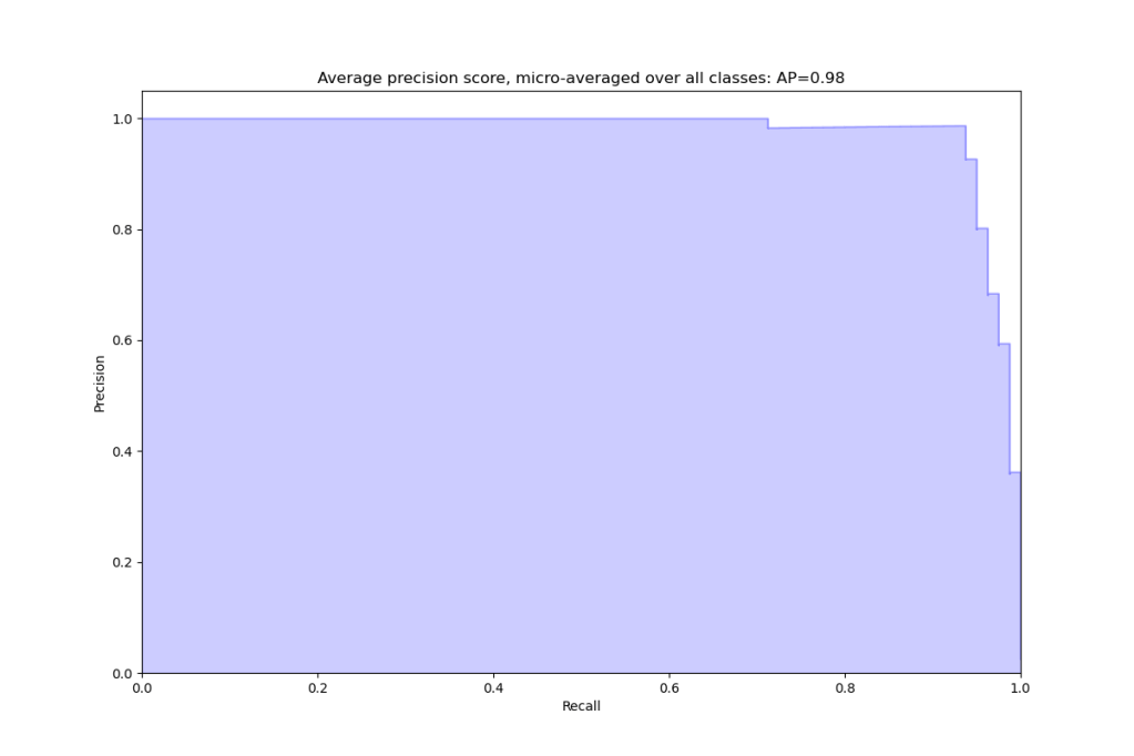
For each class
precision = dict()
recall = dict()
average_precision = dict()
for i in range(n_classes):
precision[i], recall[i], _ = metrics.precision_recall_curve(y_test_multiclass[:, i],
y_score[:, i])
average_precision[i] = metrics.average_precision_score(y_test_multiclass[:, i], y_score[:, i])
A “micro-average”: quantifying score on all classes jointly
precision[“micro”], recall[“micro”], _ = metrics.precision_recall_curve(y_test_multiclass.ravel(),
y_score.ravel())
average_precision[“micro”] = metrics.average_precision_score(y_test_multiclass, y_score,
average=”micro”)
print(‘Average precision score, micro-averaged over all classes: {0:0.2f}’
.format(average_precision[“micro”]))
Average precision score, micro-averaged over all classes: 0.98
Let’s plot the average precision (AP) score, micro-averaged over all classes
!pip install funcsigs
from funcsigs import signature
step_kwargs = ({‘step’: ‘post’}
if ‘step’ in signature(plt.fill_between).parameters
else {})
plt.figure(1, figsize=(12,8))
plt.step(recall[‘micro’], precision[‘micro’], color=’b’, alpha=0.2,
where=’post’)
plt.fill_between(recall[“micro”], precision[“micro”], alpha=0.2, color=’b’,
**step_kwargs)
plt.xlabel(‘Recall’)
plt.ylabel(‘Precision’)
plt.ylim([0.0, 1.05])
plt.xlim([0.0, 1.0])
plt.title(
‘Average precision score, micro-averaged over all classes: AP={0:0.2f}’
.format(average_precision[“micro”]))
plt.savefig(‘averageprecisionscore.png’)
- LDA+LR Cascade Pipeline
from sklearn.pipeline import Pipeline
work_flows_std = list()
work_flows_std.append((‘lda’, LinearDiscriminantAnalysis()))
work_flows_std.append((‘logReg’, LogisticRegression(C=1.0, penalty=”l2″)))
model_std = Pipeline(work_flows_std)
model_std.fit(X_train, y_train)
y_pred=model_std.predict(X_test)
print(“Accuracy score:{:.2f}”.format(metrics.accuracy_score(y_test, y_pred)))
print(“Classification Results:\n{}”.format(metrics.classification_report(y_test, y_pred)))
Accuracy score:0.96
Classification Results:
              precision    recall  f1-score   support

           0       1.00      1.00      1.00         2
           1       1.00      1.00      1.00         2
           2       0.50      1.00      0.67         2
           3       1.00      1.00      1.00         2
           4       1.00      1.00      1.00         2
           5       1.00      1.00      1.00         2
           6       1.00      1.00      1.00         2
           7       1.00      0.50      0.67         2
           8       1.00      1.00      1.00         2
           9       1.00      1.00      1.00         2
          10       1.00      1.00      1.00         2
          11       1.00      1.00      1.00         2
          12       1.00      1.00      1.00         2
          13       1.00      1.00      1.00         2
          14       1.00      1.00      1.00         2
          15       1.00      1.00      1.00         2
          16       1.00      1.00      1.00         2
          17       1.00      1.00      1.00         2
          18       1.00      1.00      1.00         2
          19       1.00      1.00      1.00         2
          20       1.00      1.00      1.00         2
          21       1.00      0.50      0.67         2
          22       1.00      1.00      1.00         2
          23       1.00      1.00      1.00         2
          24       1.00      1.00      1.00         2
          25       1.00      0.50      0.67         2
          26       1.00      1.00      1.00         2
          27       1.00      1.00      1.00         2
          28       1.00      1.00      1.00         2
          29       1.00      1.00      1.00         2
          30       1.00      1.00      1.00         2
          31       1.00      1.00      1.00         2
          32       1.00      1.00      1.00         2
          33       1.00      1.00      1.00         2
          34       1.00      1.00      1.00         2
          35       1.00      1.00      1.00         2
          36       1.00      1.00      1.00         2
          37       1.00      1.00      1.00         2
          38       0.67      1.00      0.80         2
          39       1.00      1.00      1.00         2

    accuracy                           0.96        80
   macro avg       0.98      0.96      0.96        80
weighted avg       0.98      0.96      0.96        80
- Unsupervised ML via KMeans Clusters
import scikitplot as skplt
import sklearn
from sklearn.model_selection import train_test_split
from sklearn.ensemble import RandomForestClassifier, RandomForestRegressor, GradientBoostingClassifier, ExtraTreesClassifier
from sklearn.linear_model import LinearRegression, LogisticRegression
from sklearn.cluster import KMeans
from sklearn.decomposition import PCA
import matplotlib.pyplot as plt
import sys
import warnings
warnings.filterwarnings(“ignore”)
print(“Scikit Plot Version : “, skplt.version)
print(“Scikit Learn Version : “, sklearn.version)
print(“Python Version : “, sys.version)
%matplotlib inline
Scikit Plot Version :  0.3.7
Scikit Learn Version :  1.1.3
Python Version :  3.9.16 (main, Jan 11 2023, 16:16:36) [MSC v.1916 64 bit (AMD64)]
skplt.cluster.plot_elbow_curve(KMeans(random_state=1),
X_train,
cluster_ranges=range(2, 20),
figsize=(8,6));
plt.savefig(‘elbowplot.png’)

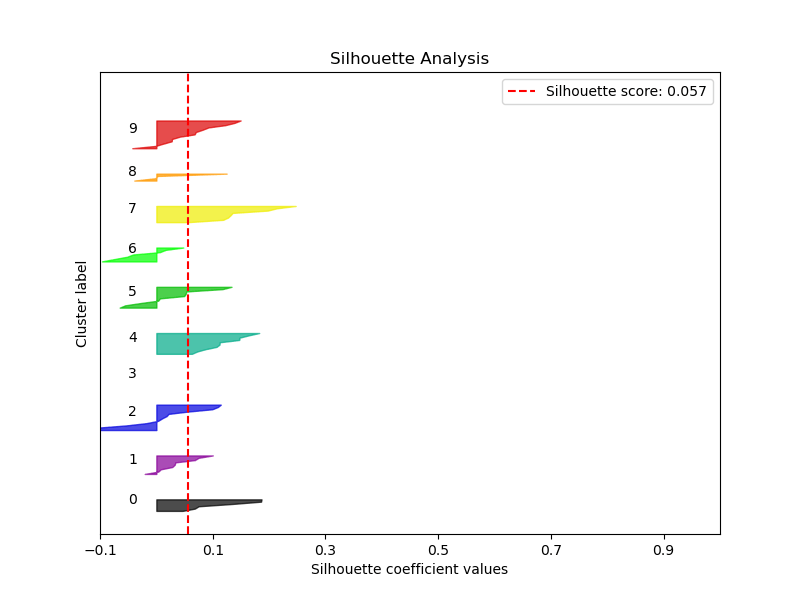
kmeans = KMeans(n_clusters=10, random_state=1)
kmeans.fit(X_train, y_train)
cluster_labels = kmeans.predict(X_test)
skplt.metrics.plot_silhouette(X_test, cluster_labels,
figsize=(8,6));
plt.savefig(‘silhouetteanalysis.png’)
- PCA Validation
pca = PCA(random_state=1)
pca.fit(X_train)
skplt.decomposition.plot_pca_component_variance(pca, figsize=(8,6));
plt.savefig(‘pcacomponentexplainedvariance.png’)

skplt.decomposition.plot_pca_2d_projection(pca, X_train, y_train,
figsize=(10,10),
cmap=”tab10″);
plt.savefig(‘pca_2d_projection.png’)

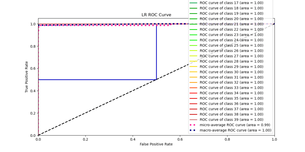
- Multi-class LR ROC and Precision-Recall Curves
log_reg=LogisticRegression(C=1.0, penalty=”l2″)
log_reg.fit(X_train, y_train)
Y_test_probs = log_reg.predict_proba(X_test)
skplt.metrics.plot_roc_curve(y_test, Y_test_probs,
title=”LR ROC Curve”, figsize=(12,6));
plt.savefig(‘LROCCURVE.png’)

skplt.metrics.plot_precision_recall_curve(y_test, Y_test_probs,
title=”LR Precision-Recall Curve”, figsize=(12,6));
plt.savefig(‘LRprecisionrecallcurve.png’)


Real-Time Webcam
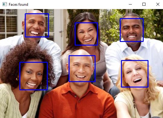
Let’s look at the image snapshot officepeople3.jpg of a live webcam session. We need the extra xml file haarcascade_frontalface_default.xml. Both files are to be copied to the local directory YOURPATH. The three-step face detection workflow is as follows
import os
os.chdir(‘YOURPATH’)
os. getcwd()
import cv2
import sys
imagePath = ‘officepeople3.jpg’
cascPath = ‘haarcascade_frontalface_default.xml’
faceCascade = cv2.CascadeClassifier(cascPath)
Read and convert image:
image = cv2.imread(imagePath)
gray = cv2.cvtColor(image, cv2.COLOR_BGR2GRAY)
Detect faces in the image:
faces = faceCascade.detectMultiScale(
gray,
scaleFactor=1.1,
minNeighbors=5,
minSize=(30, 30),
# flags = cv2.cv.CV_HAAR_SCALE_IMAGE
)
print(“Found {0} faces!”.format(len(faces)))
Show face detections:
for (x, y, w, h) in faces:
cv2.rectangle(image, (x, y), (x+w, y+h), (255, 0, 0), 2)
cv2.imshow(“Faces found”, image)
cv2.waitKey(0)
Found 6 faces!
Summary
- We have implemented and tested the iterative FR process of giving Python ML pipelines the ability to identify or verify different facial features.
- This is the three-phase process: Data Gathering, Train/Test/Validate the Recognizer, and Recognition with relevant ML error metrics.
- FR ML algorithms have tasks called multi-label classifiers.
- We use cascades to solve the problem of detecting faces into multiple stages.
- Cascades do a very rough and quick test for each block. If that block passes, does a more detailed test and so on.
- We have been able to detect who the image represents in the photo using a simple PCA + supervised ML approach by detecting, manipulating and identifying the contours of the face.
- This clearly shows how ML has rapidly taken charge in the world of AI. A day-to-day sample is Facebook, which automatically tags people found in a photo without tagging them manually.
- FR can serve as an excellent security measure for time tracking and attendance.
- FR is also cheap technology as there is less processing involved, like in other biometric techniques.
Explore More
- Comparative ML/AI Performance Analysis of 13 Handwritten Digit Recognition (HDR) Scikit-Learn Algorithms with PCA+HPO
- Case Study: Multi-Label Classification of Satellite Images with Fast.AI
- Multi-Label Keras CNN Image Classification of MNIST Fashion Clothing
Appendix The LFW Dataset
".. _labeled_faces_in_the_wild_dataset:\n\nThe Labeled Faces in the Wild face recognition dataset\n------------------------------------------------------\n\nThis dataset is a collection of JPEG pictures of famous people collected\nover the internet, all details are available on the official website:\n\n http://vis-www.cs.umass.edu/lfw/\n\nEach picture is centered on a single face. The typical task is called\nFace Verification: given a pair of two pictures, a binary classifier\nmust predict whether the two images are from the same person.\n\nAn alternative task, Face Recognition or Face Identification is:\ngiven the picture of the face of an unknown person, identify the name\nof the person by referring to a gallery of previously seen pictures of\nidentified persons.\n\nBoth Face Verification and Face Recognition are tasks that are typically\nperformed on the output of a model trained to perform Face Detection. The\nmost popular model for Face Detection is called Viola-Jones and is\nimplemented in the OpenCV library. The LFW faces were extracted by this\nface detector from various online websites.\n\n**Data Set Characteristics:**\n\n ================= =======================\n Classes 5749\n Samples total 13233\n Dimensionality 5828\n Features real, between 0 and 255\n ================= =======================\n\nUsage\n~~~~~\n\n``scikit-learn`` provides two loaders that will automatically download,\ncache, parse the metadata files, decode the jpeg and convert the\ninteresting slices into memmapped numpy arrays. This dataset size is more\nthan 200 MB. The first load typically takes more than a couple of minutes\nto fully decode the relevant part of the JPEG files into numpy arrays. If\nthe dataset has been loaded once, the following times the loading times\nless than 200ms by using a memmapped version memoized on the disk in the\n``~/scikit_learn_data/lfw_home/`` folder using ``joblib``.\n\nThe first loader is used for the Face Identification task: a multi-class\nclassification task (hence supervised learning)::\n\n >>> from sklearn.datasets import fetch_lfw_people\n >>> lfw_people = fetch_lfw_people(min_faces_per_person=70, resize=0.4)\n\n >>> for name in lfw_people.target_names:\n ... print(name)\n ...\n Ariel Sharon\n Colin Powell\n Donald Rumsfeld\n George W Bush\n Gerhard Schroeder\n Hugo Chavez\n Tony Blair\n\nThe default slice is a rectangular shape around the face, removing\nmost of the background::\n\n >>> lfw_people.data.dtype\n dtype('float32')\n\n >>> lfw_people.data.shape\n (1288, 1850)\n\n >>> lfw_people.images.shape\n (1288, 50, 37)\n\nEach of the ``1140`` faces is assigned to a single person id in the ``target``\narray::\n\n >>> lfw_people.target.shape\n (1288,)\n\n >>> list(lfw_people.target[:10])\n [5, 6, 3, 1, 0, 1, 3, 4, 3, 0]\n\nThe second loader is typically used for the face verification task: each sample\nis a pair of two picture belonging or not to the same person::\n\n >>> from sklearn.datasets import fetch_lfw_pairs\n >>> lfw_pairs_train = fetch_lfw_pairs(subset='train')\n\n >>> list(lfw_pairs_train.target_names)\n ['Different persons', 'Same person']\n\n >>> lfw_pairs_train.pairs.shape\n (2200, 2, 62, 47)\n\n >>> lfw_pairs_train.data.shape\n (2200, 5828)\n\n >>> lfw_pairs_train.target.shape\n (2200,)\n\nBoth for the :func:`sklearn.datasets.fetch_lfw_people` and\n:func:`sklearn.datasets.fetch_lfw_pairs` function it is\npossible to get an additional dimension with the RGB color channels by\npassing ``color=True``, in that case the shape will be\n``(2200, 2, 62, 47, 3)``.\n\nThe :func:`sklearn.datasets.fetch_lfw_pairs` datasets is subdivided into\n3 subsets: the development ``train`` set, the development ``test`` set and\nan evaluation ``10_folds`` set meant to compute performance metrics using a\n10-folds cross validation scheme.\n\n.. topic:: References:\n\n * `Labeled Faces in the Wild: A Database for Studying Face Recognition\n in Unconstrained Environments.\n <http://vis-www.cs.umass.edu/lfw/lfw.pdf>`_\n Gary B. Huang, Manu Ramesh, Tamara Berg, and Erik Learned-Miller.\n University of Massachusetts, Amherst, Technical Report 07-49, October, 2007.\n\n\nExamples\n~~~~~~~~\n\n:ref:`sphx_glr_auto_examples_applications_plot_face_recognition.py`\n"


Make a one-time donation
Make a monthly donation
Make a yearly donation
Choose an amount
Or enter a custom amount
Your contribution is appreciated.
Your contribution is appreciated.
Your contribution is appreciated.
DonateDonate monthlyDonate yearly
Leave a comment